Cost-efficient forest management for safeguarding Siberian flying squirrel (Pteromys volans) habitats in Central Finland

ABSTRACT

Protection of vulnerable species often creates conflicts between land use and conservation management. Particularly challenging is the case of Siberian flying squirrel (SFS; Pteromys volans). SFS favours mature forest habitats, which are often the target for logging, and therefore its protection causes opportunity costs. In our analysis a regional case study was applied as a platform to create alternative forest management scenarios. These scenarios aimed to maintain and improve SFS habitats with varying magnitudes, from no action in SFS habitat improvement to increasing the amount of suitable habitat for SFS. Stand projections for each forest management scenario were modelled with the Motti stand simulator, and the simulated stand structures were further analyzed using specific indexes with Geographic Information System (GIS) methodologies and tools to predict potential nesting and feeding habitats and connectivity for SFS. Connectivity between habitats was assessed with a Least Cost Path analysis. The results showed that some forest management scenarios were more cost-efficient than others in maintaining habitat suitability and connectivity for SFS. Further, with adjusted cutting removals (due to restrictions other than SFS habitat related, mainly recreation) an additional hectare suitable for SFS habitat was considerably more cost-efficient than without the adjustment.

KEYWORDS:

• Siberian flying squirrel
• cost-effectiveness
• simulation
• conservation

Introduction

The biodiversity in forested environments worldwide is under increasing pressure from anthropogenic resource extraction resulting in habitat loss, fragmentation, and the deterioration of extant habitats (Pimm et al. 2014). Therefore, safeguarding forest biodiversity has become one of the most important goals in multiple-use forestry (European Commission 2006). Human induced habitat loss and fragmentation are perhaps the two primary drivers of the biodiversity crisis in terrestrial ecosystems (Millennium Ecosystem Assessment 2005). Further, increased habitat fragmentation and decreased landscape connectivity often result in reduced dispersal rates (e.g. Schtickzelle et al. 2006), leading to increased isolation between populations and smaller population sizes (Diffendorfer et al. 1995). For instance, the movements of some species are directly influenced by landscape composition and configuration (Smith et al. 2011; Trapp et al. 2019). Even countries with large forest reserves and well-developed conservation programs have failed in stopping the decline of forest species populations (e.g. European Commission 2011, 2015). The boreal forests represent a third of the earth’s woodland cover but are under imminent pressure from intensive resource extraction (Wistbacka et al. 2018), which poses a major threat to the persistence of boreal species (Schmiegelow and Mönkkönen 2002).

In Fennoscandia, industrial silvicultural treatments are typically clearcuttings (Kuuluvainen et al. 2012), causing progressive deterioration of the ecological value of forests and further resulted in many forest habitats becoming endangered or near threatened (Raunio et al. 2008; Wistbacka et al. 2018). Due to clearcutting phase followed by artificial regeneration, the landscape is usually mosaic of deforested areas of even-aged naturally-regenerating stands and plantation-esque stands with declining old-growth forest patches (Kuuluvainen 2009; Santangeli et al. 2013a).

Further, reports on declines of forest-dependent taxa are growing steadily (Rassi et al. 2010). One such declining species is the Siberian flying squirrel (SFS; Pteromys volans), a vulnerable species protected under Habitats Directive 92/43/EEC within its European range encompassing Finland and to a smaller extent Estonia (Santangeli et al. 2013a). SFS’s red listed status (according to IUCN principles) implies that its habitat is warranted by legal protection in Finland. In addition to legally enforced protection, a strong understanding of species habitat requirements across the squirrel’s different life-stages is essential in order to effectively adopt protective measures into forest management practices (Wistbacka et al. 2018). New scientific information on the interaction between adaptive forest management and SFS’s habitat requirements is needed to mitigate the negative influence of habitat loss on the species (Ritchie et al. 2009).

As a “Nearly Threatened” and a flagship species in Finland (Liukko et al. 2016), SFS’s occurrence increases with the increasing average forest age, increasing volume of spruce trees (Picea abies (L.) Karst.), and there has to be large deciduous trees within the spruce forest (e.g. Reunanen et al. 2002; Santangeli et al. 2013b). On the landscape scale, the presence of agricultural fields has also been positively associated to the occurrence of SFS (Santangeli et al. 2013b), as fields occur in regions with fertile soil (Remm et al. 2017). Mixed forest structure driven by soil fertility favours SFS since alders (Alnus incana L., Alnus glutinosa L.) and birches (Betula pendula Roth., Betula pubescens Ehrh.) are important food sources, although aspen (Populus Tremula L.), Scots pine (Pinus sylvestris L.), and Norway spruce are also used as forage (Selonen and Mäkeläinen 2017). During winter and early spring, birch and alder catkins are the main food sources (Selonen et al. 2016) and SFS cache alder catkins in cavities, nest-boxes and on tree branches (Selonen and Wistbacka 2016).

In addition to food, the presence of nesting sites affects SFS habitat selection (Selonen and Hanski 2004). In Finland, SFS occupy large home-ranges: males move on average within a 60-hectare area and females within an 8-hectare area (Hanski et al. 2000). Although there is no clear effect of fragmentation on SFS (see, Lampila et al. 2009 vs. Remm et al. 2017), it is clear that open areas restrict the movements of the squirrels because they exceed the gliding capacity of SFS (Selonen and Hanski 2004). Further, responses to fragmentation are likely density-dependent and region-specific (Remm et al. 2017), and there appears to be a minimal amount of preferred forest habitat in the landscape in occupancy patterns (e.g. Reunanen et al. 2004; Remm et al. 2017).

The interaction between forest management and suitable habitats for SFS is evident: management can either destroy, maintain, or enhance habitats through manipulating the forest structure and patch connectivity (Reunanen et al. 2002; Haakana et al. 2017; Selonen and Mäkeläinen 2017). The history of forest management in Fennoscandia, and particularly in Finland, has been focused on wood production effects on the forest structure and both landscape habitat composition and configuration in a way which results in the loss and fragmentation of mature mixed spruce deciduous forests favourable for SFS habitat (Reunanen et al. 2002; Selonen and Mäkeläinen 2017). Therefore, SFS could be negatively affected by the prevailing intensive forest management of clearcutting (Santangeli et al. 2013a; Wistbacka et al. 2018). This sensitivity to clearcutting forest management practices seems to be common among flying squirrels in general due to loss of overstory trees and canopy cover (Ritchie et al. 2009).

Thus far the low success of current conservation management in protecting SFS implies poor cost-efficiency despite several management restrictions applied in SFS forests (Selonen and Mäkeläinen 2017). Along with commercial timber production forest, SFS also live in urban green areas less intensively managed for timber production (Mäkeläinen et al. 2015). An additional challenge related to this particular case study is that it represents a municipal recreation forest (e.g. Horne et al. 2005), which has resulted in a permanent decrease in the level of annual cutting removals compared to commercial forests without such restrictions on management. Additionally, it remains to be seen whether a reduction in cutting activities would have a substantially positive effect on SFS habitat potential.

To be able to assess the effect of alternative forest management regimes on SFS habitat availability, we first need to estimate stand projections and link them with SFS habitat models (Haakana et al. 2017). In this study, we produced alternative management scenarios to discover how they affect predicted suitable SFS habitats within a 30-yr time horizon. The management scenarios represent alternative goals of forest management – from pure timber production to different SFS habitat conservation treatments. Further, we assessed the trade-offs (timber revenues vs. suitable SFS habitat areas) between management scenarios in order to reveal the cost-efficiency of protecting SFS habitats. To our knowledge such an analysis is the first of a kind (cf. Haakana et al. 2017). Therefore, we also provide guidelines to protect suitable SFS habitats with a cost-efficient manner in which the benefit (i.e. increasing the amount of suitable SFS habitat) is highest for any given cost (i.e. losses in timber revenues; Margules and Pressey 2000).

Material and methods

Forest data

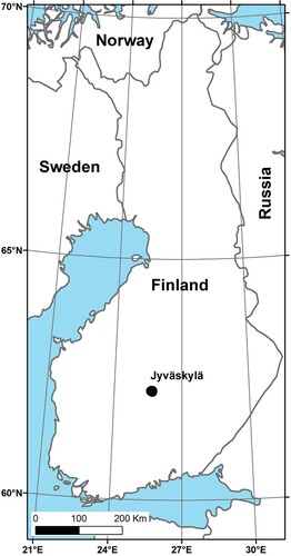
The study area encompassed approximately 558 ha of municipal forest land administered by the city of Jyväskylä in south-central Finland (Figure 1). These publicly owned forests were located within the city limits and used for forestry and recreational purposes (hiking, berry picking, and winter sports). Mainly due to recreational use by the public, recent forest management activities in the study area have been lower compared to commercial forests of the region, wherein 2300 m³ annual harvesting removals occur in multi-use forests (corresponding to ca. 4.1 m³ ha⁻¹ year⁻¹, which is lower than the average in the region, 5.1 m³ ha⁻¹ year⁻¹; Finnish forest statistics 2020). Within our study area, 1.3 ha regeneration cuttings, 23.3 ha thinnings and 2.0 ha tending of young stands were annually operated.

Figure 1. Location of the study area.

We applied stand-wise (e.g. site fertility, location and main tree species) and stratum-wise data (stem number, basal area, mean diameter, mean height), totalling of 504 individual forest stands. According to these data, most of the stands were spruce dominated on the medium rich sites (Table 1). The proportion of the stands ≥60 or ≥100 years of age were 45% and 32% of the total area, respectively. Aspen and birch species represented 2% and 13% of the stand volume, respectively (Table 1) and are important deciduous species in SFS habitat. However, the large-diameter aspen and birch stems were obtained only in ca. 1% and 13% of the stands, respectively. Furthermore, 194 stands out of 504 had cutting restrictions in the initial data due to municipal recreation forest management.

Table 1. Average stand characteristics of the study area in Jyväskylä.

Fertility	Number of stands	Area, ha	Area, %	Stand age, yrs (average, range)	Stand volume, m^3 ha^−1 (average, range)	Tree species distribution, % of the stand volume
						Pine	Spruce	Birch	Aspen
1	10	10.9	2.0	108 (44–149)	150 (68–246)	21	41	22	17
2	197	202.3	36.3	71 (0–141)	241 (0–490)	16	68	14	2
3	251	297.3	53.3	71 (0–151)	213 (0–402)	34	52	12	1
4	35	35.9	6.4	78 (0–155)	133 (0–288)	77	15	7	1
5	9	11	2.0	57(0–135)	66 (0–151)	94	2	4	0
6	2	0.8	0.1	58 (0–115)	51 (0–101)	100	0	0	0
All	504	558.1	100	72 (0–155)	214 (0–490)	29	57	13	2

Fertility improves with descending order: 1 presents the most fertile site type. Site fertility levels based on the Finnish site type classes from the most fertile (class 1) to the most barren, class 6 (Tonteri et al. 1990).

Calculating SFS indexes

We build a set of indexes based on stand-structure to predict potential SFS nesting habitat. Flying squirrels favour mature or old-growth Norway spruce-dominated forests with deciduous trees (Hanski 1998) and they mainly use cavities for nesting (Hanski et al. 2000). Michon (2014) reported that the average diameter at breast height (DBH) for cavity trees was 27.3 cm (SD = 7.6) in managed boreal forests of Middle Sweden, in an area similar in size to our study area. A correlation analysis between age and DBH in our data showed that the stands were 64 years old when DBH was 20 cm (y = 16.775e^0.0672DBH, R²= 0.5148). Applying all these criteria, we defined nesting habitat as stands where the proportion of spruce is >50% of stand volume, age of spruce trees is ≥60 years, and the proportion of deciduous tree species is >1% of stand volume. Additionally, abreast with the above-mentioned criteria we categorized a stand suitable for nesting according to the tree species and tree size: (i) suitable forests at present with large aspen stems (≥20 cm DBH), (ii) forests developing suitable within 30 yrs with medium-size aspen stems (15–19.9 cm DBH), or (iii) suitable forests at present with large birch stems (≥25 cm DBH). We did not use other deciduous tree species as a criterion due to lack of data. As a result, there were 68 stands classified as the most preferred SFS habitat in our study area.

The occupancy of SFS in a stand is dependent on the amount of preferred habitat in the surrounding area (Hurme et al. 2005) and the connectivity among these habitat patches (Reunanen et al. 2002). Therefore, one aim in forest planning scenarios was to maintain connectivity among preferred habitats during the planning period. To account for connectivity, we calculated another set of indexes for each stand to describe stand’s suitability as a corridor or stepping stone (see Selonen and Hanski 2003) for the movements of SFS. SFS can use relatively young forests for movement between habitat patches (Selonen and Hanski 2003) and we defined the minimum average tree height for a SFS corridor as 10 m.

We calculated connections between all pairs of nesting stands by using the Cost Path tool in ArcGIS Desktop 10.6.1. The tool calculates the Least Cost Path (LCP) distance between selected targets over a cost surface. LCP is a resistance-based method that calculates theoretical costs for an individual to move in a certain type of habitat and other landscape cover types (Diniz et al. 2020). The basic idea in LCP analysis is to find routes between habitat patches that minimize the cumulative cost of movement. For our analysis, the landscape was divided into 16 m × 16 m size raster cells and each cell was given a cost (resistance) value (i.e. the cost for an individual animal to traverse it; Table 2) thus forming a cost surface as a result. As the real costs for movement between different habitat types are not known, we followed the common practice to use SFS habitat suitability as a starting point to define costs for movement (Diniz et al. 2020). Maximum dispersal distance refers to reported maximum dispersal distances from their natal habitats which has been reported to be at maximum about 6600 m (Selonen and Hanski 2006). We set the maximum dispersal to 7500 m, which enables the path traverse the whole study area. All the other LCP cost definitions are given in Table 2.

Table 2. Costs and maximum traversing distances for forests and other habitats used in Least Cost Path (LCP) analysis.

Class number	Habitat class name	Cost	Description
1	The most preferred habitat (nesting habitat)	1	Technical cost of 1 was assigned for the best habitat type to avoid Manhattan type of path shapes in resulting paths within class 1 stands
2	The most preferred habitat type in future	22	Maximum moving distance 7500 m
3	Movement habitat	32	Forests with average tree height >10 m, do not fulfill criteria for habitat types 1 or 2, maximum moving distance 5000 m
4	Movement barrier	2000	Forests with average tree height < 10 m, openings, fields, maximum moving distance 64 m, allows for additional 1000 m moving in movement habitat
5	Water	4000	All types of waters, maximum moving distance 32 m, allows for additional 1000 m moving in movement habitat
6	Roads	2000	Maximum moving distance 64 m, allows for additional 1000 m moving in movement habitat

LCP was calculated between every combination of two nesting habitats and the number of paths traversing through stands was used as a weight for stands in scenarios. The most preferred habitat type in future refers to stands with similar characteristics as in the most preferred stands but they probably fulfill the age and DBH of trees of class 1 criteria during the simulation period of 30 years. Maximum distances of movement barriers, waters and roads were adjusted such that they allowed for additional 1000 m movement in moving habitat.

For each nesting stand pair, an LCP was calculated over the cost surface and the resulting LCP was added to an LCP network. Next, an overlay analysis was performed between the LCP network and forest stands. Forest stands containing LCP corridors were then classified according to the number of connections traversing them by using following values: (1) Number of connections ≥500 (connects about 44% of nesting stands), (2) number of connections ≥200 (connects 66% of nesting stands), or (3) number of connections greater than 50 (connects 90% of nesting stands). Cut point values for the number of connections were selected such that they divide the distribution as close as possible to 50%, 75% and 90% in stand connection data.

Both sets of SFS indexes (nesting habitats and corridors) were applied in formulating different forest management scenarios (Table 3). We calculated SFS-indexes at the onset of the simulation (year 0) and at the end of the 30-yr period to take into account how alternative forest management scenarios affect SFS habitat availability across time. The rationale of alternative forest management scenarios was to assess potential impacts of forest management on habitat suitability for SFS (see Haakana et al. 2017), and further to reveal trade-offs between losses of timber revenues and habitat suitability.

Table 3. Forest management scenarios with stand characteristics, connectivity criteria and actions allowed.

Forest management scenario	Stands characteristics, connectivity and actions allowed
	Stand characteristics for nesting habitat	Actions	Criteria for connectivity	Actions
SG1	Not relevant^a	No restrictions	Not relevant^a	No restrictions
Forest management scenarios contributing SFS habitats, SG2−SG11
SG2	Large aspen^b [4]	No cuttings^c	No criteria	No restrictions
SG3	Large aspen and/or medium-sized aspen^d [19]	No cuttings	No criteria	No restrictions
SG4	Large aspen and/or medium-sized aspen and/or large birch^e [68]	No cuttings	No criteria	No restrictions
SG5	Large aspen [4]	No cuttings	Number of connections, NOC > 500 [29]	Only thinnings^f
SG6	Large aspen [4]	No cuttings	NOC > 500 or NOC > 200 [67]	Only thinnings
SG7	Large aspen [4]	No cuttings	NOC > 500, NOC > 200 or NOC > 50 [143]	Only thinnings
SG8	Large aspen and/or medium-sized aspen and/or large birch [68]	No cuttings	NOC > 500 [29]	Only thinnings
SG9	Large aspen and/or medium-sized aspen and/or large birch [68]	No cuttings	NOC > 500 or NOC > 200 [67]	Only thinnings
SG10	Large aspen and/or medium-sized aspen and/or large birch [68]	No cuttings	NOC > 500, NOC > 200 or NOC > 50 [143]	Only thinnings
SG11	Large aspen and/or medium-sized aspen and/or large birch [68]	No cuttings	NOC > 500, NOC > 200 or NOC > 50 [143]	No cuttings

Allowed cuttings are presented for each management scenario SG1–SG11. Calculated SFS indexes were applied both at the onset of simulations as well as at the end of the 30-yr simulations. Numbers in brackets indicate the number of individual stands with corresponding stand characteristics and connectivity criteria at the onset of the simulations, year 2021.

^a In SG1 each stand is managed according to silvicultural guidelines which currently ignore SFS habitats.

^b Large aspen indicates that in a stand there are aspen stems/trunks with minimum diameter exceeding 22 cm (at breast height).

^c No cuttings indicate that neither thinnings nor clear cuttings are allowed in such stands.

^d Medium-sized aspen corresponds to a diameter of < 20 cm for aspen.

^e Large birch requires a birch stem larger than 22 cm at breast height.

^f Only thinnings allowed in such stands, no clear cutting.

Forest management scenarios

The base scenario (SG1) represents forestry practice where stands are managed strictly according to silvicultural guidelines (for guidelines, see Äijälä et al. 2019). For instance, thinnings were based on basal area, BA (when a BA associated with a particular dominant height exceeds, a thinning is conducted) while clear cuttings were based on diameter or age limits. In stand reestablishment after clear cutting, artificial regeneration (either planting or sowing) was favoured over natural regeneration (e.g. a seed tree method), and all stands were assumed to be managed according to the principles applied in rotation forestry (RF) in contrast to continuous cover forestry (CCF). Therefore, this scenario corresponds to forest management focusing only on sustainable timber production.

The flying-squirrel scenarios (SG2-SG11) represent different forest management options to conserve suitable habitat for SFS. Constraints on forest management were set via connectivity or nesting habitats requirements or both (Table 2). In general, any logging (either thinning or clear cutting) in nest habitat was not allowed, whereas thinning in connectivity corridors were allowed, with the exception of the SG11 scenario. Subsequently, the constraints on forest management were tightened so that the number of potential nesting habitat and corridors (based on SFS indexes described above) increased from scenario SG2 to scenario SG11 (Table 3). At the same time, the array of silvicultural actions narrowed towards SG11 (Table 3).

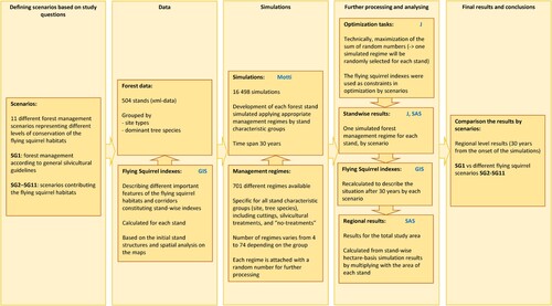
Technically, we constructed SG2–SG11 scenarios according to a specific optimization procedure (for technical details see Lappi and Lempinen 2014) in which the calculated SFS indexes served as constraints so that management scenario SG11 represents a solution without any management activity (i.e. no cuttings allowed; Table 3). A technical overview of dataset, indexes, simulations, and optimization procedure to construct forest management scenarios is presented in Figure 2. For instance, in SG11 there are a total of 211 stands in which cuttings are prohibited, whereas in SG1 all 504 stands can be managed without any restrictions related to potential SFS habitat (Table 3).

Figure 2. Overview of dataset, indexes, simulations, and optimization procedure to construct management scenarios. Applied software presented in blue font. ArcGIS Desktop 10.6.1 (ESRI 2018) was used in the spatial analyses and Motti Stand Simulator (Salminen et al. 2005; Hynynen et al. 2015) in the simulations. Further analyses were carried out with SAS (ver 9.4, X64_10PRO platform) and J (Lappi and Lempinen 2014) software.

Stand projections

We used Motti stand simulator (Hynynen et al. 2015; Juutinen et al. 2018; Ahtikoski et al. 2021) to model alternative forest management scenarios SG1-SG11. In this study Motti stand simulator version 6.0.3 was applied. Motti stand simulator (henceforth Motti) is a tool for predicting forest development and dynamics in certain conditions and after application of silvicultural treatments (Hynynen et al. 2014). Motti includes a combination of several models, such as tree growth, mortality, and the effects of silvicultural treatments at stand level. Models produce predictions for all dominant tree species in forests across Finland (Salminen et al. 2005; Hynynen et al. 2014; Hynynen et al. 2015). We created the input data for the Motti using both stand-wise information of the site fertility, as well as location and stratum-wise information by tree species (e.g. stem number, basal area, mean diameter, mean height). Specifically, we predicted the development of each stand according to several a priori management regimes for stand characteristic groups i.e. dominant tree species, site type, and location – see Figure 2. Under these different management regimes, stands were managed with alternative silvicultural treatments and/or cuttings by varying the timings and intensities of the treatments. Basically, we simulated from four to 74 alternative management regimes for each individual stand (Figure 2) depending on the stand characteristic group (Figure 2). The rationale was to cover a wide range of management options for later analysis of SFS habitat suitability. All simulated regimes were based on rotation forestry, RF (i.e. even-aged management) and thinnings were conducted from below. Technically, for each stand (belonging to a particular stand characteristic group – see Figure 2) we altered the timings of the thinnings (expressed as a dominant height), the intensity of the thinnings (expressed as a decrease in basal area) and the timing for clear cutting (expressed either by average diameter or stand age). In brief, each stand was simulated according to altered values for the timings of thinnings, timing of clear cutting and the choice of regeneration method (artificial or natural), resulting in numerous management regimes for that particular stand (for a detailed description of identical technical lay out, see Haikarainen et al. 2021, Table 2). Further, for each stand we also simulated a “no-treatments” alternative. In total there were 16 489 individual simulations (management regimes) covering the study area (558 ha) which consists of numerous stand characteristic groups (Figure 2). In all simulations we predicted tree growth for a 30-year time period.

From these simulated regimes based on the different silvicultural treatments, only one regime for each stand was selected to present a particular forest management scenario. This selection was based on optimization procedure (Figure 2), wherein one management regime for each stand was chosen to fulfil a particular forest management scenario (see Table 3). The rationale of such an approach was to create alternative forest management scenarios in which the management regimes would together correspond to the principles of a particular scenario. Furthermore, the optimization ensured that the forest management scenarios would be genuinely different from each other due to different constraints associated with the scenarios (see Tables 2 and 3) and multiple alternative management regimes to choose from on the stand-level. We generated a random number for each simulated regime indicating that an individual regime had an identical probability to be selected via the “optimized” the random number (for identical application of random numbers in optimization, see Hynynen et al. 2015; Haikarainen et al. 2021). As a result, we could fine-tune the management regimes corresponding to the forest management scenarios by varying the constraints in the optimization framework. Finally for each forest management scenario, we inputted the results into GIS software, and SFS indexes were recalculated for the 30-year end simulation and compared to pre-simulation indexes (Figure 2). Finally, with recalculated SFS indexes and Net Present Values, NPVs associated with each stand in each forest management scenario, we were able to compare the impacts of alternative forest management scenarios on SFS habitat suitability with monetary trade-offs, i.e. losses in timber revenues. Net Present Value, NPV is a standard concept to represent economic preferences in environmental science (Knoke et al. 2020). It is based on discounting to calculate present values for future net benefits so that net benefits occurring at different time points in evolving time become comparable (Knoke et al. 2020).

Financial data

In assessing NPV for each stand in each forest management scenario, we applied stumpage prices and silvicultural costs according to nominal time series from 2002–2016. The rationale for applying time series observation was to capture several business cycles so that the calculated average would include both peak and bottom prices and costs. We considered the last year of time series (2016) as the most recent year since there was a change in methodology post-2016. We then adjusted the nominal time series of stumpage prices and silvicultural costs by the cost-of-living index (Official Statistics Finland 2017) to attain real prices and costs for the selected time period (Table 4).

Table 4. Stumpage prices and silvicultural costs (in real terms) applied in assessing the NPV for forest management scenarios SG1-SG11.

Stumpage prices	Sawlogs, € m^−3	Pulpwood, € m^−3	Energywood, € m^−3
First commercial thinning	Pine: 42.19 Spruce: 42.70 Birch: 37.00	12.70 14.72 12.23
Intermediate thinnings	50.99 50.69 41.85	15.88 19.38 15.10
Final cutting	60.38 60.30 49.44	18.76 23.73 18.18
All cuttings and tree species			Stems: 4.24 Crowns: 3.40 Stumps: 1.43
Silvicultural costs
Labour cost of planting Material costs of planting Seeding Mounding Disc trenching Patch scarification Early cleaning Precommercial thinning Clearing of a thinning area Ditch network maintenance Fertilization	0.16–0.20 €/seedling^a 0.19–0.24 €/ seedling^a 224.5 € ha^−1 355.5 € ha^−1 196.0 € ha^−1 313.9 € ha^−1 35 € hour^−1^b 35 € hour^−1 35 € hour^−1 185 € ha^−1 320 € ha^−1

^a Unit costs per seedling depends on tree species (planting density).

^b Unit cost per hour, total costs calculated with time consumption models resulting in € ha⁻¹.

Financial analyses

Stand-level Motti simulations were used to analyze tree growth, timber production and financial performance of forest management scenarios. We used cutting incomes of thinnings and clearcuttings as well as silvicultural costs to calculate NPV (for methodology, see Knoke and Moog 2005; Hökkä et al. 2017) according to the time horizon of 30 years. The NPV was assessed according to: $NP{V}_a=\sum _{s=1}^S\left[\sum _{i=0}^T{b}^{t_i}\left(\sum _{k=1}^{K}C{I}_{ki}^s-\sum _{m=1}^{M}S{C}_{mi}^s\right)\right]$where NPVa is net present value for forest management scenario a, a = SG1, … , SG11, s denotes an individual stand, s = 1,..,504, ti is a year within the time horizon i∈ {0, … 30} s.t. T = 30, b is the discount factor (b = 1/(1 + r) where r is the interest rate in real terms), CIki indicates cutting income from the kth thinning at year ti, s.t. K indicates a clear-cutting and SCmi is a cost for a silvicultural action m at year ti.

Sensitivity analysis

Since the level of annual cuttings in the study area was lower on average compared to other sites in the region, we conducted a sensitivity analysis. The lower level of annual cuttings was due to restrictions not related to SFS habitat management (e.g. recreational issues, biodiversity management) in the study area. In the sensitivity analysis, we adjusted the realized level of annual cuttings indicating considerably smaller timber harvests than in SG scenarios. For instance, the annual cuttings of SG1 without prevailing restrictions were ca. 2 600 m³ while with restrictions (i.e. adjusted) ∼1 600 m³ in the study area.

Results

The effects of modelled forest management scenarios on the volume of birches and aspen as well as on the number of connections between SFS habitats was clear but moderate (Table 5). For instance, the average volume for SG1 was 23.1 birches and 1.1 m³ ha⁻¹ aspen while for SG 11 the values were 27.4 and 1.6 m³ ha⁻¹, respectively (Table 5). The area of suitable SFS forests after 30 years fluctuated considerably between the forest management scenarios (Table 5). For example, the area of suitable SFS forests is as high as 140.3 hectares for forest management scenario SG11 after 30 years while for SG1 the corresponding area is only 87.2 hectares (i.e. 38% less) after the same time period (Table 5). Figure 3 illustrates suitable SFS forests and corridors associated with SG1 and SG11 after 30 years of management. For instance, the number of potential corridors according to SG11 distinctively exceeds the number of corridors of SG1, indicating a much better potential for SFS to survive.

Figure 3. Suitable SFS forests (dark colour) and corridors (lines) associated with management scenario SG1 (a) and SG11 (b) after a 30 year-period.

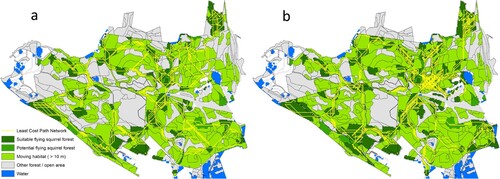
Table 5. Average stocking and volumes of birches and aspen and total number of connections associated with forest management scenarios.

Forest management scenario	Average stocking (of which birches and aspen volumes), m^3 ha^−1	Area of suitable SFS forests at the end of time horizon^b, hectares
SG1	196.4 (23.1 and 1.1)^a	87.2
SG2 SG3 SG4	197.8 (23.1 and 1.2) 202.7(23.3 and 1.4) 213.2 (24.2 and 1.4)	90.1 101.1 120.4
SG5 SG6 SG7	207.9 (23.9 and 1.2) 220.6 (25.6 and 1.2) 236.5 (27.0 and 1.5)	103.1 120.5 139.8
SG8 SG9 SG10	217.6 (24.7 and 1.4) 225.4 (25.8 and 1.4) 236.9 (27.0 and 1.5)	124.2 131.8 140.3
SG11	237.8 (27.4 and 1.6)	140.3

^a The first value, 23.1 represents the volume of birches, and the second, 1.1 of aspen, m³ ha⁻¹.

^b The end of the time horizon corresponds to year 30.

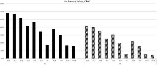
As expected, forest management scenario SG1 produced the highest NPV, regardless of the interest rate applied (Figure 4). For instance, the SG1 NPV was over 2000 € ha⁻¹ higher than the SG11 NPV when 2% interest rate was applied (Figure 4). Interestingly, SG7 and SG10 resulted in similar NPVs. This is due to the fact that the amount of aspen in the study area was minimal (see Table 5) so that the large aspen criterion of SG7 becomes practically irrelevant. This results in that SG7 and SG10 are almost identical with respect to stand structures of nesting habitats (see Table 3), given that other criteria between SG7 and SG10 are identical.

Figure 4. Net Present Values (NPV) associated with forest management scenarios SG1-SG11, when 2% and 4% interest rates applied.

Since the SG1 scenario produced the highest NPV and resulted the smallest total area (ha) of suitable SFS forests as expected, it was logical to set SG1 as the base scenario for comparing the cost-efficiency of actively managing for SFS habitat. The cost efficiency of increasing the area of suitable SFS habitat fluctuated considerably between forest management scenarios (Table 6). For instance, according to SG2 an additional hectare of suitable SFS forest would cost 14 081 € ha⁻¹ while the cost would be 21 801 € ha⁻¹ for SG7 with an interest rate of 2% (Table 6). With 4% interest rate, the corresponding costs are slightly smaller (Table 6). This is mainly due to different timing of the cuttings associated with SG1 in relation to other forest management scenarios, resulting in an anomaly in which higher interest rate produces a smaller cost, € ha⁻¹. However, the differences between 2% and 4% interest rate are not significant (Table 6).

Table 6. Cost of an additional hectare suitable for SFS, € ha⁻¹.

Forest management scenario	Cost with 2% interest rate, € ha−^1	Cost with 4% interest rate, € ha^−1
SG2	14 081	14 145
SG3	12 580	12 026
SG4	13 897	13 398
SG5	20 187	18 916
SG6	19 810	17 769
SG7	21 801	18 957
SG8	15 461	14 668
SG9	17 607	16 046
SG10	21 741	18 929
SG11	22 127	19 251

Interest rate 2% and 4%.

Sensitivity analysis

As anticipated the cost of an additional hectare of suitable SFS habitat was on average lower with adjusted cutting removals (Table 7). On the other hand, the differences of suitable SFS habitat between management scenarios were considerably smaller with adjusted cutting removals (Table 7) compared to original setting (Table 6). For simplicity, results of the sensitivity analysis are presented only for management scenarios SG1, SG3, SG5, SG8 and SG11. For instance, SG5 adjusted the cost of an additional hectare of suitable SFS habitat was less than 6 000 € ha⁻¹ (Table 7), whereas in the original analysis the cost was over 20 000 € ha⁻¹ with 2% interest rate (Table 6). On the other hand, the cost was higher for an adjusted SG11 (Table 7) compared to original result (Table 6).

Table 7. Cost of an additional hectare suitable for SFS, € ha⁻¹ when adjusted cutting removals applied.

Forest management scenario	Cost with 2% interest rate, € ha^−1	Cost with 4% interest rate, € ha^−1	Area of suitable SFS forests at the end of time horizon, hectares
SG3adjusted	12 176	11 388	153.5
SG5adjusted	5 584	5 423	154.7
SG8adjusted	9 947	8 448	167.2
SG11adjusted	25 948	20 628	165.6

Interest rate 2% and 4%. Area of suitable SFS forests also depicted at the end of the time horizon, i.e. 30 years. For BAUadjusted the suitable SFS forests covered 149.1 hectares at year 30 (cf. Table 5: SG1 87.2 ha).

Discussion

This study tackled assessing the cost-efficiency of providing suitable habitats for SFS in silviculturally management areas. Alternative forest management scenarios were ranked according to their cost-efficiency in producing suitable SFS habitats and connections between them, including monetary estimates (i.e. NPV), into the assessment is a new approach (cf. Kurttila et al. 2002; Ritchie et al. 2009; Haakana et al. 2017). By including financial aspects into the comparison of alternative forest management scenarios, it allows an evaluation of the cost of simultaneously managing for SFS and utilizing the forests for timber production, further aiding decision-making balancing economic and conservation objectives.

The impact of alternative forest management scenarios on suitable SFS habitats is complex (Haakana et al. 2017). For instance, an earlier study (Reunanen et al. 2002) argued that it would be difficult to determine whether the age of the forest was important for SFS habitat selection, because SFS was not present in some forests despite them being old-growth forests. Average forest variables mask out the variation within forests, e.g. the presence of large trees, which introduces random uncertainty when defining SFS habitats with forest planning data. Further, a recent study (Jokinen et al. 2019) indicated that the average winter temperature had the largest predictive power for SFS occurrences – the winter temperature is hardly a variable to be manipulated by forest management. However, the living conditions of SFS can be improved by e.g. saving adjacent or nearby SFS habitats from cuttings (Kurttila et al. 2002). In addition, forest planning data have been shown to be useful in estimating the suitability of SFS habitats (Hurme et al. 2005), and forest management has a direct effect on SFS nesting habitat patches with more intensive management negatively impacting these habitats (Wistbacka et al. 2018). Another important factor for suitable SFS habitats is landscape configuration (Ritchie et al. 2009; Smith et al. 2013;Trapp et al. 2019), which can be influenced by forest management.

A limitation of this study is it was based on stand projection models simulated according to growth and yield models and incorporated into a decision-support software (Salminen et al. 2005; Hynynen et al. 2015). Simulation is a powerful modelling method (Mota and Flores 2020), but it has several pitfalls (see Koivisto 2017), wherein which interpretation is possibly the most critical here. An interpretation pitfall results when stand projections are produced by simulations to describe stand structure, which is further applied in creating indexes to predict (e.g. potential nesting habitats). As a result, critical distance to the simulation results may be lost (see Barth et al. 2012).

The similarity between SG7 and SG10 forest management scenarios (Tables 5 and 6) with respect to suitable SFS habitat and cost-efficiency indicates that there seems to be synergy between the stand structure and connectivity criteria, especially when suitable habitats are scarce in the landscape. The stand structure parameters used in this study (age, tree species mixture, DBH) and the amount of high-quality stands associated with SFS nesting habitat has been shown to predict the occurrence of SFS (Reunanen et al. 2002; Hurme et al. 2005). Due to differences in landscape structure among areas, models explaining the occupancy of SFS at one site do not necessarily have inference across the landscape (Hurme et al. 2005). Additionally, there was a lack of SFS data from our study area and therefore only within-stand parameters based of known SFS ecology were used in our study.

SFS are able to efficiently use a matrix of habitats for movements and can also cross narrow open areas (Selonen and Hanski 2003). However, there is no quantitative information about the importance of different connecting habitats between nesting stands, thus our LCP method and criteria to classify stands was based on theoretical assumptions generally used in landscape connectivity modelling (Diniz et al. 2020). However, although being rather generic, we believe that both stand-wise and landscape-level connectivity criteria for SFS were feasible enough to be applied as simulation criteria. The financial results (cost-efficiency) according to adjusted and original cutting removals differed considerably (Table 6 vs. Table 7). This emphasizes the importance of local conditions and multipurpose forestry: how forest ecosystem management could be utilized to meet the societal demands (i.e. recreation) and to ensure ecological integrity for wildlife (Asbjornsen et al. 2022). In the case study region, it seems that some synergy with recreation and SFS habitats could be achieved – this can be supported by the fact that on average the cost of an additional hectare suitable for SFS (€ ha-1) was slightly less with adjusted cutting removals than without the adjustment, depending on the status of a municipal recreation forest. Another intriguing result was that the cost of an additional hectare suitable for SFS was surprisingly high compared to the cost of protecting other species (e.g. caribou habitat; Yemshanov et al. 2020), the cost per hectare for biodiversity conservation (Vaezin et al. 2022), the costs due to NATURA 2000 management restrictions (Jacobsen et al. 2013), or the value of non-wood forest products (i.e. NWFP; Lovrić et al. 2020). However, the difference can be explained by the fact that SFS nesting habitat occurs in mature stands with high stocking indicating high opportunity costs.

With regard to main results and safeguarding SFS habitats raises another question: what amount of additional suitable habitat and corridors would actually maintain or increase the SFS occurrence. For instance, this study employed a variety of forest management scenarios, including some which were more cost-effective than others. However, more cost-effective scenarios did not increase absolute hectares of SFS suitable habitat nor increased connectivity compared to less cost-effective scenarios.

In Finland, SFS occurrence increases with average forest age, volume of spruce trees and share of deciduous trees within the spruce forest (Reunanen et al. 2002; Santangeli et al. 2013b). Further, the preference for fertile soil and mixed forest structure (spruce with deciduous trees) is explained by the food habits of SFS: alder and birch are important food sources especially in winter and spring, but also aspen, pine and spruce are used as forage (Selonen et al. 2016; Selonen and Mäkeläinen 2017). Thus, SFS occurrence is linked to the availability of deciduous trees. As a result, there has been a debate on whether conservation management would focus on enhancing habitat quality rather than enhancing landscape connectivity (e.g. Mortelliti et al. 2011; Selonen and Mäkeläinen 2017). Selonen and Hanski (2003) argued that conservation policies for SFS in southern Finland should aim for maintaining high quality stands for SFS rather than focusing on connectivity, because most of the forests in southern Finland are not isolated from each other by large open areas. Our data do not allow for comparing the importance of habitat quality and landscape connectivity for SFS but our results show that it is possible to include both elements in forest planning and to compare cost-effectiveness of these measures.

Conclusions

New knowledge on cost-effective SFS conservation management is urgently needed, given the success of conservation management for this species to date. This study provides information on the cost-effectiveness of SFS conservation management options. Although the results are ad hoc, they contribute current literature by introducing monetary values for alternative management options conserving SFS habitats, potentially helping decision making related to planning conservation for SFS habitats.

Disclosure statement

No potential conflict of interest was reported by the author(s).

Correction Statement

This article has been corrected with minor changes. These changes do not impact the academic content of the article.

References

- Ahtikoski A, Laitila J, Hilli A, Päätalo M-L. 2021. Profitability of the first commercial thinning, a simulation study in northern Finland. Forests. 12:1389. doi:10.3390/f12101389.
- Äijälä O, Koistinen A, Sved J, Vanhatalo K, Väisänen P. 2019. Metsänhoidon suositukset [Silvicultural guidelines] (In Finnish).
- Asbjornsen H, Wand Y, Ellison D, Ashcraft CM, Atallah SS, Mayer A, Altamirano M, Yu P. 2022. Multi-targeted payments for the balanced management of hydrological and other forest ecosystem services. Forest Ecol Manag. 522(2022):120482. doi:10.1016/j.foreco.2022.120482.
- Barth R, Meyer M, Spitzner J. 2012. Typical pitfalls of simulation modelling – lessons learned from armed forces and business. J Artif Soc Soc Simul. 15(2):5. http://jasss.soc.surrey.ac.uk/15/2/5.html.
- Diffendorfer JE, Gaines MS, Holt RD. 1995. Habitat fragmentation and movements of three small mammals (Sigmodon, Microtus, and Peromyscus). Ecology. 76:827–839.
- Diniz MF, Cushman SA, Machado RB, Júnior PDM. 2020. Landscape connectivity modeling from the perspective of animal dispersal. Landsc Ecol. 35:41–58. doi:10.1007/s10980-019-00935-3.
- ESRI. 2018. ArcGIS desktop: release 10.6. Redlands, CA: Environmental Systems Research Institute.
- European Commission. 2006. EU biodiversity action plan. Halting the loss of biodiversity by 2010 – and beyond – sustaining ecosystem services for human well-being. [accessed 2012 March 21]. http://ec.europa.eu/environment/nature/biodiversity/comm2006/index_en.htm.
- European Commission. 2011. Our life insurance, our natural capital: an EU biodiversity strategy to 2020. COM/2011/244 final. Brussels, 3.5.2011.
- European Commission. 2015. The mid-term review of the EU biodiversity strategy to 2020. COM/2015/0478 final. Brussels, 2.10.2015.
- Finnish forest statistics. 2020. Peltola, A. (Editor-in-chief), Räty, M., Sauvula-Seppälä, T., Torvelainen, J., Uotila, E., Vaahtera, E. and Ylitalo, E. (Eds.) 198 pages. http://urn.fi/URN:ISBN:978-952-380-107-3.
- Haakana H, Hirvelä H, Hanski IK, Packalen T. 2017. Comparing regional forest policy scenarios in terms of predicted suitable habitats for the Siberian flying squirrel (Pteromys volans). Scand J Forest Res. 32(2):185–195. doi:10.1080/02827581.2016.1221991.
- Haikarainen S, Huuskonen S, Ahtikoski A, Lehtonen M, Salminen H, Siipilehto J, Korhonen KT, Hynynen J, Routa J. 2021. Does juvenile stand management matter? Regional scenarios of the long-term effects on wood production. Forests. 12(1):17.
- Hanski IK. 1998. Home ranges and habitat use in the declining flying squirrel Pteromys volans in managed forests. Wildlife Biol. 4:33–46. doi:10.2981/wlb.1998.013.
- Hanski IK, Stevens PC, Ihalempiä P, Selonen V. 2000. Home-range size, movements, and nest-size use in the Siberian flying squirrel, Pteromys Volans. J Mamm. 81:798–809.
- Hökkä H, Salminen H, Ahtikoski A, Kojola S, Launiainen S, Lehtonen M. 2017. Long-term impact of ditch network maintenance on timber production, profitability and environmental loads at regional level – a simulation study. Forestry. 90(2):234–246. doi:10.1093/forestry/cpw045.
- Horne P, Boxall PC, Adamowicz WL. 2005. Multiple-use management of forest recreation sites: a spatially explicit choice experiment. Forest Ecol Manag. 207:189–199. doi:10.1016/j.foreco.2004.10.026.
- Hurme E, Mönkkönen M, Nikula A, Nivala V, Reunanen P, Heikkinen T, Ukkola M. 2005. Building and evaluating predictive occupancy models for the Siberian flying squirrel using forest planning data. Forest Ecol Manag. 216:241–256.
- Hynynen J, Salminen H, Ahtikoski A, Huuskonen S, Ojansuu R, Siipilehto J, Lehtonen M, Eerikäinen K. 2015. Long-term impacts of forest management on biomass supply and forest resource development: a scenario analysis for Finland. Europ J Forest Res. 134:415–431. doi:10.1007/s10342-014-0860-0.
- Hynynen J, Salminen H, Huuskonen S, Ahtikoski A, Ojansuu R, Siipilehto J, Lehtonen M, Rummukainen A, Kojola S, Eerikäinen K. 2014. Scenario analysis for the biomass supply potential and the future development of Finnish forest resources. Working Papers of the Finnish Forest Research Institute 302. http://www.metla.fi/julkaisut/workingpapers/2014/mwp302.htm.
- Jacobsen JB, Vedel SE, Thorsen BJ. 2013. Assessing costs of multifunctional NATURA 2000 management restrictions in continuous cover beech forest management. Forestry. 2013(86):575–582. doi:10.1093/forestry/cpt023.
- Jokinen M, Hanski I, Numminen E, Valkama J, Selonen V. 2019. Promoting species protection with predictive modelling: effect of habitat, predators and climate on the occurrence of the Siperian flying squirrel. Biol Conserv. 230:37–46. doi:10.1016/j.biocon.2018.12.008.
- Juutinen A, Ahtikoski A, Lehtonen M, Mäkipää R, Ollikainen M. 2018. The impact of a short-term carbon payment scheme on forest management. Forest Policy Econ. 90(2018):115–127. doi:10.1016/j.forpol.2018.02.005.
- Knoke T, Gosling E, Paul C. 2020. Use and miuse of the net present value in environmental studies. Ecol Econ. 174(2020):106664. doi:10.1016/j.ecolecon.2020.106664.
- Knoke T, Moog M. 2005. Timber harvesting versus forest reserves – producer prices for open-use areas in German beech forests (Fagus sylvatica L.). Ecol Econ. 52:97–110.
- Koivisto M. 2017. Pitfalls in modelling and simulation. 6th Internat. Young Scientists Conference in HPC and simulation, YSC 2017, 1-3 Nov. 2017, Kotka, Finland. Proc Comput Sci. 119 (2017):8–15. doi:10.1016/j.procs.2017.11.154.
- Kurttila M, Pukkala T, Loikkanen J. 2002. The performance of alternative spatial objective types in forest planning calculations: a case for flying squirrel and moose. Forest Ecol Manag. 166(2002):245–260.
- Kuuluvainen T. 2009. Forest management and biodiversity conservation based on natural ecosystem dynamics in Northern Europe: the complexity challenge. Ambio. 38:309–315.
- Kuuluvainen T, Tahvonen O, Aakala T. 2012. Even-aged and uneven-aged forest management in Boreal Fennoscandia: a review. Ambio. 7:720–737.
- Lampila S, Kvist L, Wistbacka R, Orell M. 2009. Genetic diversity and population differentiation in the endangered Siberian flying squirrel (Pteromys volans) in a fragmented landscape. Europ J Wildl Res. 55:397–406.
- Lappi J, Lempinen R. 2014. A linear programming algorithm and software for forest-level planning problems including factories. Scand J Forest Res. 29(Suppl. 1):178–184. doi:10.1080/02827581.2014.886714.
- Liukko UM, Henttonen H, Hanski IK, Kauhala K, Kojola I, Kyheröinen EM. 2016. The 2015 red list of Finnish mammal species. Helsinki: Finnish Environment Institute. http://hdl.handle.net/10138/159434.
- Lovrić M, Da Re R, Vidale E, Prokofieva I, Wong J, Pettenella D, Verkerk PJ, Mavsar R. 2020. Non-wood forest products in Europe – A quantitative overview. For Policy Econ. 116(2020):102175. doi:10.1016/j.forpol.2020.102175.
- Mäkeläinen S, Schrader M, Hanski IK. 2015. Factors explaining the occurance of the Siberian flying squirrel in urban forest landscape. Urban Ecosyst. 18:223–238.
- Margules CR, Pressey RL. 2000. Systematic conservation planning. Nature. 405:243–253.
- Michon S. 2014. Comparison of tree cavity abundance and characteristics in managed and unmanaged Swedish boreal forest. Swedish University of Agricultural Sciences. Faculty of Forest Science. Examensarbete i ämnet bioogi 2014:13. 26 p. https://stud.epsilon.slu.se/7417/7/michon_s_141015.pdf.
- Millennium Ecosystem Assessment. 2005. Ecosystems and human well-being: current state and trends. Washington, DC: World Resources Institute.
- Mortelliti A, Amori G, Capizzi D, Cervone C, Fagiani S, Pollini B, Boitani L. 2011. Independent effects of habitat loss, habitat fragmentation and structural connectivity on the distribution of two arboreal rodents. J Appl Ecol. 48:163–172.
- Mota M, Flores I. 2020. Revisiting the flaws and pitfalls using simulation in the analysis of aviation capacity problems. Case Stud Transp Policy. 8(2020):67–75. doi:10.1016/j.cstp.2018.03.004.
- Official Statistics of Finland. 2017. Consumer price index [e-publication]. January 2017, Appendix table 3. Cost-of-living Index 1951:10=100. [accessed 15 November 2018]. http://www.stat.fi/til/khi/2017/01/khi_2017_01_2017-02-20_tau_003_en.html.
- Pimm SL, Jenkins CN, Abell R, Brooks TM, Gittleman JL, Joppa LN, Raven P, Roberts CM, Sexton JO. 2014. The biodiversity of species and their rates of extinction, distribution, and protection. Science. 344:1246752. doi:10.1126/science.1246752.
- Rassi P, Hyvärinen E, Juslén A, Mannerkoski I. 2010. The 2010 Red List of Finnish species, Helsinki.
- Raunio A, Schulman A, Kontula T. 2008. Suomen luontotyyppien uhanalaisuus. [Threatened biotypes in Finland] (In Finnish).
- Remm J, Hanski I, Tuominen S, Selonen V. 2017. Multilevel landscape utilization of the Siberian flying squirrel: scale effects on species habitat use. Ecol Evol. 7(20):8303–8315.
- Reunanen P, Mönkkönen M, Nikula A. 2002. Habitat requirements of the Siberian flying squirrel in northern Finland: comparing field survey and remote sensing data. Ann Zool Fenn. 39:7–20.
- Reunanen P, Mönkkönen M, Nikula A, Hurme E, Nivala V. 2004. Assessing landscape thresholds for the Siberian flying squirrel. Ecol Bull. 51:277–286.
- Ritchie LE, Betts MG, Forbes G, Vernes K. 2009. Effect of landscape composition and configuration on northern flying squirrels in a forest mosaic. Forest Ecol Manag. 257:1920–1929. doi:10.1016/j.foreco.2009.01.028.
- Salminen H, Lehtonen M, Hynynen J. 2005. Reusing legacy FORTRAN in the MOTTI growth and yield simulator. Comput Electr Agric. 49:103–113. doi:10.1016/j.compag.2005.02.005.
- Santangeli A, Hanski IK, Mäkelä H. 2013b. Integrating multi-source forest inventory and animal survey data to assess nationwide distribution and habitat correlates of the Siberian flying squirrel. Biol Conserv. 157:31–38.
- Santangeli A, Wistbacka R, Hanski IK, Laaksonen T. 2013a. Ineffective enforced legislation for nature conservation: a case with Siperian flying squirrel and forestry in a boreal landscape. Biol Conserv. 157:237–244. doi:10.1016/j.biocon.2012.09.012.
- Schmiegelow FKA, Mönkkönen M. 2002. Habitat loss and fragmentation in dynamic landscapes: avian perspectives from the boreal forest. Ecol Appl. 12:375–389.
- Schtickzelle N, Mennechez G, Baguette M. 2006. Dispersal depression with habitat fragmentation in the bog fritillary butterfly. Ecology. 87:1057–1065.
- Selonen V, Hanski IK. 2003. Movements of the flying squirrel Pteromys volans in corridors and in matrix habitat. Ecography. 26:641–651.
- Selonen V, Hanski IK. 2004. Young flying squirrels (Pteromys volans) dispersing in fragmented forests. Beh Ecol. 15:564–571.
- Selonen V, Hanski IK. 2006. Habitat exploration and use in dispersing juvenile flying squirrels. J Anim Ecol. 75:1440–1449. doi:10.1111/j.1365-2656.2006.01168.x.
- Selonen V, Mäkeläinen S. 2017. Ecology and protection of a flagship species, the Siperian flying squirrel. Hystrix. 28(2):134–146. doi:10.4404/hystrix-28.2-12328.
- Selonen V, Wistbacka R. 2016. Siberian flying squirrels do not anticipate future resource abundance. BMC Ecol. 16:51.
- Selonen V, Wistbacka R, Korpimäki E. 2016. Food abundance and weather modify reproduction of two arboreal squirrel species. J Mamm. 97:1376–1384.
- Smith MJ, Betts MG, Forbes GJ, Kehler DG, Bourgeois MC, Flemming SP. 2011. Independent effects of connectivity predict homing success by northern flying squirrel in a forest mosaic. Landsc Ecol. 26(5):709–721.
- Smith MJ, Forbes GJ, Betts MG. 2013. Landscape configuration influences gap-crossing decisions of northern flying squirrel (Glaucomys sabrinus). Biol Conserv. 168:176–183.
- Tonteri T, Hotanen J-P, Kuusipalo J. 1990. The Finnish forest site type approach: ordination and classification studies of mesic forest sites in southern Finland. Vegetation. 87:85–98.
- Trapp SE, Day CC, Flaherty EA, Zollner PA, Smith WP. 2019. Modeling impacts of landscape connectivity on dispersal movements of northern flying squirrels (Gaucomys sabrinus griseifrons). Ecol Model. 394:44–52. doi:10.1016/j.ecolmodel.2018.12.025.
- Yemshanov D, Haight RG, Liu N, Parisien M-A, Barber Q, Koch FH, Burton C, Mansuy N, Campioni F, Choudhury S. 2020. Assessing the trade-offs between timber supply and wildlife protection goals in boreal landscapes. Can J Forest Res. 50(2020):243–258. doi:10.1139/cjfr-2019-0234.
- Vaezin SMH, Marage D, Garcia S. 2022. Cost-effectiveness of Natura 2000 forest contracts for biodiversity conservation. Can J Forest Res. doi:10.1139/cjfr-2021-0204.
- Wistbacka R, Orell M, Santangeli A. 2018. The tragedy of the science-policy gap – revised legislation fails to protect an endangered species in a managed boreal landscape. Forest Ecol Manag. 422:172–178. doi:10.1016/j.foreco.2018.04.017.