What is fair? Proxy discrimination vs. demographic disparities in insurance pricing

Abstract

Discrimination and fairness are major concerns in algorithmic models. This is particularly true in insurance, where protected policyholder attributes are not allowed to be used for insurance pricing. Simply disregarding protected policyholder attributes is not an appropriate solution as this still allows for the possibility of inferring protected attributes from non-protected covariates, leading to the phenomenon of proxy discrimination. Although proxy discrimination is qualitatively different from the group fairness concepts discussed in the machine learning and actuarial literature, group fairness criteria have been proposed to control the impact of protected attributes on the calculation of insurance prices. The purpose of this paper is to discuss the relationship between direct and proxy discrimination in insurance and the most popular group fairness axioms. We provide a technical definition of proxy discrimination and derive incompatibility results, showing that avoiding proxy discrimination does not imply satisfying group fairness and vice versa. This shows that the two concepts are materially different. Furthermore, we discuss input data pre-processing and model post-processing methods that achieve group fairness in the sense of demographic parity. As these methods induce transformations that explicitly depend on policyholders' protected attributes, it becomes ambiguous whether direct and proxy discrimination is, in fact, avoided.

Keywords:

• Discrimination
• indirect discrimination
• proxy discrimination
• fairness
• input preprocessing
• output post-processing
• optimal transport
• Wasserstein distance

1. Introduction

1.1. Problem context

For legal and societal reasons, there are several policyholder attributes that are not allowed to be used in insurance pricing (Avraham et al., 2014; Chibanda, 2021; European Commission, 2012; European Council, 2004; Prince & Schwarcz, 2020); for instance European law does not allow the use of information on sex in insurance pricing. Furthermore, ethnicity is a critical attribute that is typically viewed as a protected characteristic. In the actuarial and insurance literature, Charpentier (2022), Frees and Huang (2022) and Xin and Huang (2021) give extensive overviews on the potential use (direct or indirect) of policyholders' protected attributes and the implications for insurance prices, while Avraham et al. (2014), Prince and Schwarcz (2020) and Maliszewska-Nienartowicz (2014) provide legal viewpoints on this topic. Closely related is the recent report of the European Insurance and Occupational Pension Authority (EIOPA) (EIOPA, 2021), which discusses governance principles towards an ethical and trustworthy use of artificial intelligence in the insurance sector.

A critical observation from this literature is that just ignoring (being unaware of) protected information does not guarantee a lack of discrimination in pricing. In the presence of statistical associations between covariates used in pricing, it can occur that protected attributes are inferred from non-protected covariates, which thus act as undesirable proxies for, e.g. sex or ethnicity. As a result, the calculated insurance prices are subject to proxy discrimination; for a wide-ranging overview of this idea see (Tschantz, 2022).

Defining, identifying and addressing proxy discrimination presents a number of interrelated challenges and here we outline but a few. First, such discrimination need not be intentional, as the inference of protected attributes can take place implicitly through the fitting procedure of a predictive model. The complexity of models often used in insurance pricing can make this inference process quite opaque to the user. Second, the non-protected covariates implicitly used as proxies cannot just be removed from models, as, besides their proxying effect, they are typically considered legitimate predictors of policyholders' risk (e.g. smoking status can correlate with sex, while at the same time having a clear and established link to health outcomes). Third, proxy discrimination relates to the way that prices are calculated and does not necessarily imply adverse outcomes for any protected demographic group – in fact, in some situations proxy discrimination can mask rather than exacerbate demographic disparities (see Remark 9 in Lindholm et al. (2022).)

The third challenge above can be a source of confusion when discussing indirect discriminatory effects, as it relates to the complex relation between proxy discrimination and notions of group fairness, which place requirements on the joint statistical behaviour of insurance prices, protected attributes and actual claims (for example, independence between prices and protected attributes is known as demographic parity). Common definitions of indirect discrimination appear to require – and maybe even conflate with each other – both the proxying of protected attributes and an adverse impact on protected groups; see (Maliszewska-Nienartowicz, 2014), but also the broader discussion of Barocas et al. (2019), Chapter 4.

There have been several approaches to prevent proxy discrimination, including restrictions in the use of covariates, discussed in Section 6 of Frees and Huang (2022). More technical approaches and price adjustments include: a counter factual approach drawing from causal inference, see see (Araiza Iturria et al., 2022; Charpentier, 2022; Kusner et al., 2017); the probabilistic approach of Lindholm et al. (2022) focussing specifically on implicit inferences; and the projection method of Frees and Huang (2022). The latter approach finds itself within in a broader literature which considers adjustments to covariates, which produce independence of protected attributes from non-protected covariates; see also (Grari et al., 2022). On the face of it, this seems an attractive proposition: by breaking the dependence between protected attributes and their potential proxies, proxy discrimination is prevented. In other words: satisfying a group fairness perspective may also have the additional beneficial effect of addressing proxy discrimination. In the sequel, we will take a critical perspective to this particular rationale.

1.2. Aims and outline of the paper

In this paper, we aim to investigate the relationship between proxy discrimination – and the requirement to avoid it – and notions of group fairness. In particular, we will focus on the question of whether standard notions of group fairness (namely: demographic parity, equalized odds, and predictive parity) are consistent with avoiding proxy discrimination. This is a pertinent question, not least in the context of literature advocating the former as a solution to the latter.

In Section 2, we provide a technical definition of avoiding proxy discrimination as an individual fairness property. Individual fairness, broadly, requires that policyholders with the same characteristics receive the same premium (Charpentier, 2022; Dwork et al., 2012). In our context, we require that whether or not policyholder profiles are treated as equivalent should not hinge upon the dependence structure between protected attributes and non-protected covariates. We show through examples how standard unawareness pricing, arising from optimal claims prediction by ignoring protected information, leads to proxy discrimination, and how this issue can be addressed by the approach of Lindholm et al. (2022).

Then, we turn our attention to the compatibility of the individual fairness property of avoiding proxy discrimination with standard group fairness properties. We show that avoiding proxy discrimination does not imply satisfying any of the three group fairness properties considered. Conversely, satisfying demographic parity does not imply avoiding proxy discrimination. These results indicate that neither of the two requirements of group fairness or avoiding proxy discrimination is strictly stronger then the other; hence the former cannot be viewed as a quick fix for the latter. As these results are negative, they are derived by designing concrete (counter-)examples that demonstrate potential trade-offs and incompatibilities.

In Section 3, we discuss in more detail the impact that strategies to effect group fairness have on insurance prices, focussing specifically on demographic parity. The theory of optimal transport has recently been promoted to make statistical models fair, via its application in input pre-processing and model post-processing methods, see (Chiappa et al., 2020; del Barrio et al., 2019); an early application of these ideas in an insurance context w.r.t. creating gender-neutral policies in life insurance using mean-field approximations can be found in Example 5.1 of Djehiche and Lofdahl (2016). We study these pre- and post-processing methods, and conclude that they may be helpful tools for achieving fairness objectives in insurance pricing. Specifically, model post-processing, which is more frequently used in machine learning, is simpler to apply and allows for optimal modelling choices from the perspective of predictive accuracy. However, model post-processing can lead to results that are not easily explainable to insurance customers and policymakers. In addition, the adjustments made by these methods depend on the statistical relations between protected attributes and non-protected covariates. As these relations are often driven by portfolio composition rather than causal relations, their strength and direction remains portfolio-specific. This means that any adjustments (e.g. to model inputs) in order to achieve group fairness will have to be different from insurer to insurer. Such arbitrariness is hard to imagine in practice, for both regulatory and commercial reasons.

Furthermore, the extent to which the resulting prices can be considered free of discrimination is a matter of interpretation. Focusing on the case where model inputs are transformed to achieve independence, these adjustments are explicit functions of protected attributes and hence subject to direct discrimination. Unless the transformed inputs have an interpretation that is justifiable in its own right, we would end up in a paradoxical situation where proxy discrimination appears addressed (by independence between transformed protected and unprotected attributes), at the price of introducing direct discrimination. But this of course does not make sense, since the whole idea of avoiding proxy discrimination is conceptually predicated on the lack of direct discrimination.

In Section 4, we discuss our overall conclusions and further aspects of the problem. Mathematical results are proved in Appendix 1.

1.3. Relation to the machine learning literature

The issues we address in this paper from an insurance perspective are closely related to extensive discussions in the machine learning literature; for wide overviews of those discussions see (Barocas et al., 2019; Mehrabi et al., 2019; Tschantz, 2022). One particular difference of the discussions of fairness in the insurance pricing and machine learning contexts is that, in the former, responses of predictive models are discrete numerical or continuous, while in the latter they are typically binary/categorical. This means that one cannot assume that proofs and technical arguments developed in the machine learning literature on the relation between different notions of fairness necessarily transfer to the insurance context. Furthermore, the regulatory emphasis in insurance is more on avoiding direct and indirect (or proxy) discrimination, rather than comparing the outcomes on different demographic groups (European Commission, 2012; European Council, 2004).

We consider proxy discrimination as a type of individual fairness – since its focus is on the way similar policyholders should be treated – and we introduce a suitable notion of similarity. Our perspective on proxy discrimination is essentially the same as omitted variable bias; see (Mehrabi et al., 2019; Tschantz, 2022). We note that a substantial variety of alternative notions of proxy discrimination exist and these are typically formulated via the rich framework of causal inference, e.g. (Kilbertus et al., 2017; Kusner et al., 2017; Qureshi et al., 2016). In contrast, we make no assumptions regarding causality. There are three reasons for this. First, our focus is on indirect inference of protected attributes and this is an issue of statistical association, rather than causality. Second, the statistical relations between covariates are often not the result of any causal relations, but instead artefacts of the composition of insurance portfolios. Third, any causal relations that do exist between covariates are not necessarily well understood in practice, particularly in high-dimensional insurance pricing applications. Hence our approach is motivated by a mix of conceptual and pragmatic arguments that apply in the insurance context.

Substantial literature exists on the incompatibility of different notions of fairness, see for example the seminal contribution of Kleinberg et al. (2016) and the related discussion by Hedden (2021). Our contribution to this literature thus consists of demonstrating incompatibility of avoiding proxy discrimination with group fairness notions, from an insurance perspective. In a sense, such incompatibility is not particularly surprising, given the rather different scope of individual and group fairness. The potential conflict between those two classes of fairness criteria is discussed in Binns (2020) and Friedler et al. (2016), using, respectively, discursive and technical arguments but reaching consistent conclusions: that such conflicts demonstrate the need to clarify ideas about justice and the particular types of harm that should be prevented in specific contexts. While we do not examine the moral foundations of the technical fairness criteria, this is a conclusion we support. More practically, trade-offs between individual and group fairness are operationalized by reflecting them within model fitting processes, see for example (Awasthi et al., 2020; Lahoti et al., 2019; Zemel et al., 2013), noting that these papers do not specifically consider proxy discrimination as a type of individual (un)fairness.

Finally, the applications of methods from Optimal Transport has received prominence both in the machine learning literature, see (Chiappa et al., 2020; del Barrio et al., 2019), and more recently in actuarial science, e.g. (Charpentier et al., 2023). Our contribution to this strand of literature is primarily conceptual. We show how the incompatibility between avoiding proxy discrimination and group fairness manifests through the generation of directly discriminatory prices, when optimal transport methods are deployed to achieve demographic parity in insurance. Furthermore, we highlight the communication challenges associated with the transformations of model inputs and outputs.

2. Discrimination and fairness in insurance pricing

2.1. Proxy discrimination

To set the stage, we fix a probability space $(\mathrm{\Omega },\mathcal{F},\mathbb{P})$ with $\mathbb{P}$ describing the real world probability measure. We consider the random triplet $(Y,\mathit{X},\mathit{D})$ on this probability space. The response variable Y describes the insurance claim that we try to predict (and price). The vector $\mathit{X}$ describes the non-protected covariates (non-discriminatory characteristics), and $\mathit{D}$ describes the protected attributes (discriminatory characteristics). We assume that the partition into non-protected covariates $\mathit{X}$ and protected attributes $\mathit{D}$ is given exogenously, e.g. by law or by societal norms and preferences. We use the distribution $\mathbb{P}(Y,\mathit{X},\mathit{D})$ to describe an insurance portfolio and its claims, in particular, the random selection of a policyholder from the insurance portfolio, based on their characteristics, is given by the distribution $\mathbb{P}(\mathit{X},\mathit{D})$. Different insurance companies may have different insurance portfolio distributions $\mathbb{P}(\mathit{X},\mathit{D})$, and this insurance portfolio distribution typically differs from the overall population distribution in a given society because the insurance penetration is not uniform across the entire population. For simplicity, in this paper, we assume that the protected attributes $\mathit{D}$ are discrete and finite, only taking values in a finite set $\mathfrak{D}$.

In our context, concern for proxy discrimination arises from the understanding that even when the protected attributes $\mathit{D}$ are not used explicitly in pricing, they may still be used implicitly, because the pricing mechanisms deployed may include inference of $\mathit{D}$ from the non-protected covariates $\mathit{X}$. Hence, we require that insurance prices do not depend on the conditional distribution $\mathbb{P}(\mathit{D}\mid \mathit{X})$, such that a modification of that conditional distribution does not impact the individual prices. To formalize this concern, we first note that the distribution $\mathbb{P}$ is specific to a particular portfolio and insurance company. Let $\mathcal{P}$ be the set of all distributions over $(Y,\mathit{X},\mathit{D})$, such that any alternative insurance portfolio can be identified with a distribution $\mathbb{Q}\in \mathcal{P}$; one may think of $\mathbb{Q}$ as a modification of the portfolio distribution $\mathbb{P}$ or as another portfolio in the same idealized insurance market. Further, assume that $\mathit{X}$ takes values in a set $\mathcal{X}$, i.e. $\mathit{X}(\omega )\in \mathcal{X}$ for all $\omega \in \mathrm{\Omega }$. To start with, we consider proxy discrimination as a property of pricing functionals, defined as follows.

Definition 2.1

A pricing functional π is a mapping $\pi :\mathcal{X}\times \mathcal{P}\to \mathbb{R}$, such that for a portfolio $\mathbb{P}\in \mathcal{P}$, a policyholder with non-protected covariates $\mathit{x}\in \mathcal{X}$ is charged the insurance price $\pi (\mathit{x},\mathbb{P})$.

Note that, by construction, a pricing functional as defined above avoids direct discrimination since $\mathit{D}$ is not an explicit input to it. Avoiding proxy discrimination is a more stringent requirement, given as follows.

Definition 2.2

A pricing functional π on $\mathcal{X}\times \mathcal{P}$ avoids proxy discrimination if for any two portfolios $\mathbb{P},\mathbb{Q}\in \mathcal{P}$ that satisfy $\mathbb{P}(Y|\mathit{X},\mathit{D})=\mathbb{Q}(Y|\mathit{X},\mathit{D})$, $\mathbb{P}(\mathit{D})=\mathbb{Q}(\mathit{D})$ and $\mathbb{P}(\mathit{X})=\mathbb{Q}(\mathit{X})$, we have (1) $\pi (\mathit{X},\mathbb{P})=\pi (\mathit{X},\mathbb{Q}),\mathbb{P}-\mathrm{a}.\mathrm{s}.$(1)

Definition 2.2 of (lack of) proxy discrimination requires that in comparable insurance portfolios, prices should be identical. Comparability means that the portfolio distributions $\mathbb{P}$ and $\mathbb{Q}$ should be identical in all aspects apart from the dependence structure between $\mathit{D}$ and $\mathit{X}$, which is precisely the source of potential proxy discrimination. We may thus view the property of avoiding proxy discrimination as a particular form of individual fairness. That is, broadly, the requirement that policyholders with similar profiles regarding non-protected covariates $\mathit{X}$, receive in similar circumstances the same premium (Charpentier, 2022; Dwork et al., 2012). In the current context ‘similar circumstances’ refers to the insurance portfolios having the same structure, except for the dependence between the protected attributes $\mathit{D}$ and the non-protected covariates $\mathit{X}$. This dependence is insurance company specific and originates from the specific structure of the insurance portfolio.

In Definition 2.2 no specific pricing (or predictive) model is assumed – the definition can be applied to any functional of non-protected covariates and portfolio distribution. We note that a pricing functional violating (1(1) $\pi (\mathit{X},\mathbb{P})=\pi (\mathit{X},\mathbb{Q}),\mathbb{P}-\mathrm{a}.\mathrm{s}.$(1) ) in general does not allow us to conclude that such violations will be material in the context of a specific portfolio. To talk about materiality of proxy discrimination we need to consider a reference portfolio structure ${\mathbb{P}}^{\perp \perp }$ that is comparable to $\mathbb{P}$. By convention, we will choose ${\mathbb{P}}^{\perp \perp }$ such that under that measure $(\mathit{X},\mathit{D})$ are independent.

Definition 2.3

Proxy discrimination is material for the pricing functional π and the portfolio $\mathbb{P}$, if, for the measure ${\mathbb{P}}^{\perp \perp }$ with ${\mathbb{P}}^{\perp \perp }(Y,\mathit{X},\mathit{D})=\mathbb{P}(Y|\mathit{X},\mathit{D})\mathbb{P}(\mathit{X})\mathbb{P}(\mathit{D})$ it holds that (2) $\mathbb{P}(\pi (\mathit{X},\mathbb{P})\ne \pi (\mathit{X},{\mathbb{P}}^{\perp \perp }))>0.$(2)

The positive probability in (2(2) $\mathbb{P}(\pi (\mathit{X},\mathbb{P})\ne \pi (\mathit{X},{\mathbb{P}}^{\perp \perp }))>0.$(2) ) is calculated with respect to the distribution of $\mathit{X}$ which is the same under $\mathbb{P}$ and ${\mathbb{P}}^{\perp \perp }$. This formulation aims to avoid assigning materiality to scenarios where $\pi (\mathit{x},\mathbb{P})\ne \pi (\mathit{x},{\mathbb{P}}^{\perp \perp })$ for policies with $\mathit{X}=\mathit{x}$ that do not actually occur in the portfolio.

Our aim is to examine standard types of insurance prices from the perspective of proxy discrimination.

2.2. Discrimination-free insurance prices

Best-estimate price: For insurance pricing, one aims at designing a regression model that describes the conditional distribution of Y, given the explanatory variables $(\mathit{X},\mathit{D})$. Moreover, the main building block for technical insurance prices is the conditional expectation of claims, given the policyholder characteristics. This motivates the following definition.

Definition 2.4

For a portfolio $\mathbb{P}$ the best-estimate price of Y, given full information $(\mathit{X},\mathit{D})$, is given by (3) $\mu (\mathit{X},\mathit{D},\mathbb{P}):={\mathbb{E}}_{\mathbb{P}}[Y|\mathit{X},\mathit{D}].$(3)

This price is called ‘best-estimate’ because it has minimal mean squared error (MSE), i.e. it is the most accurate predictor for Y, given $(\mathit{X},\mathit{D})$, in the $L^2(\mathbb{P})$-sense; for simplicity, we assume that all considered random variables are square-integrable with respect to $\mathbb{P}$.

In general, the best-estimate price directly discriminates because it uses the protected attributes $\mathit{D}$ as an input, see (3(3) $\mu (\mathit{X},\mathit{D},\mathbb{P}):={\mathbb{E}}_{\mathbb{P}}[Y|\mathit{X},\mathit{D}].$(3) ). As such, it does not provide a pricing functional in the sense of Definition 2.1.

Unawareness prices : The simplest response to the direct discrimination of best-estimate prices is to obtain a pricing functional by conditioning on the non-protected covariates $\mathit{X}$ only. This approach corresponds to the concept of fairness through unawareness (FTU) in machine learning, motivating the following definition.

Definition 2.5

For a portfolio $\mathbb{P}$ the unawareness price of Y, given $\mathit{X}$, is defined by (4) $\mu (\mathit{X},\mathbb{P}):={\mathbb{E}}_{\mathbb{P}}\left[Y|\mathit{X}\right].$(4)

The unawareness price does not directly discriminate because it does not use protected attributes $\mathit{D}$ as explicit inputs. However, the unawareness price is generally not free from proxy discrimination, as it allows implicit inference of $\mathit{D}$ through the tower property (5) $\mu (\mathit{X},\mathbb{P})=\sum _{\mathit{d}\in \mathfrak{D}}\mu (\mathit{X},\mathit{d},\mathbb{P})\mathbb{P}(\mathit{D}=\mathit{d}|\mathit{X}).$(5) From Equation (5(5) $\mu (\mathit{X},\mathbb{P})=\sum _{\mathit{d}\in \mathfrak{D}}\mu (\mathit{X},\mathit{d},\mathbb{P})\mathbb{P}(\mathit{D}=\mathit{d}|\mathit{X}).$(5) ) it is apparent that a modification of the conditional distribution $\mathbb{P}(\mathit{D}|\mathit{X})$ would generally impact the calculation of $\mu (\mathit{X},\mathbb{P})$ and Equation (1(1) $\pi (\mathit{X},\mathbb{P})=\pi (\mathit{X},\mathbb{Q}),\mathbb{P}-\mathrm{a}.\mathrm{s}.$(1) ) will not generally be satisfied. If there is statistical dependence (association) between $\mathit{X}$ and $\mathit{D}$ with respect to $\mathbb{P}$, unawareness prices implicitly use this dependence for inference of $\mathit{D}$ from $\mathit{X}$; in Example 2.12, below, we illustrate this inference on an explicit example.

Nonetheless, in practice one still needs to establish whether, under the unawareness price and for a specific portfolio distribution $\mathbb{P}$, proxy discrimination is material. Hence, we need to compare $\mu (\mathit{X},\mathbb{P})$, given in (5(5) $\mu (\mathit{X},\mathbb{P})=\sum _{\mathit{d}\in \mathfrak{D}}\mu (\mathit{X},\mathit{d},\mathbb{P})\mathbb{P}(\mathit{D}=\mathit{d}|\mathit{X}).$(5) ), to the corresponding formula under ${\mathbb{P}}^{\perp \perp }$, given by (6) $\mu (\mathit{X},{\mathbb{P}}^{\perp \perp })={\mathbb{E}}_{{\mathbb{P}}^{\perp \perp }}[Y\mid \mathit{X}]=\sum _{\mathit{d}\in \mathfrak{D}}\mu (\mathit{X},\mathit{d},{\mathbb{P}}^{\perp \perp })\mathbb{P}(\mathit{D}=\mathit{d}).$(6) The comparison of formulas (5(5) $\mu (\mathit{X},\mathbb{P})=\sum _{\mathit{d}\in \mathfrak{D}}\mu (\mathit{X},\mathit{d},\mathbb{P})\mathbb{P}(\mathit{D}=\mathit{d}|\mathit{X}).$(5) ) and (6(6) $\mu (\mathit{X},{\mathbb{P}}^{\perp \perp })={\mathbb{E}}_{{\mathbb{P}}^{\perp \perp }}[Y\mid \mathit{X}]=\sum _{\mathit{d}\in \mathfrak{D}}\mu (\mathit{X},\mathit{d},{\mathbb{P}}^{\perp \perp })\mathbb{P}(\mathit{D}=\mathit{d}).$(6) ) highlights that there are two necessary conditions for proxy discrimination becoming material for $\mu (\mathit{X},\mathbb{P})$; note that $\mu (\mathit{X},\mathit{d},\mathbb{P})=\mu (\mathit{X},\mathit{d},{\mathbb{P}}^{\perp \perp })$ by assumption. First, we need to have, for some $\mathit{X}$, a conditional probability (7) $\mathbb{P}(\mathit{D}=\mathit{d}|\mathit{X})\ne \mathbb{P}(\mathit{D}=\mathit{d})\mathrm{for}\mathrm{some}\mathit{d}\in \mathfrak{D},$(7) i.e. we need to have dependence between $\mathit{X}$ and $\mathit{D}$ that allows us to (partly) infer the protected attributes $\mathit{D}$ from the non-protected covariates $\mathit{X}$, such that $\mathit{X}$ is used as a proxy for $\mathit{D}$. Second, the functional $\mathit{d}\mapsto \mu (\mathit{X},\mathit{d})$ needs to have a sensitivity in $\mathit{d}$, otherwise, if (8) $\mu (\mathit{X},\mathit{d},\mathbb{P})\equiv \mu (\mathit{X},\mathbb{P})\mathrm{for}\mathrm{all}\mathit{d}\in \mathfrak{D},$(8) the inference potential from $\mathit{X}$ to $\mathit{D}$ is not exploited in the construction of $\mu (\mathit{X})$, and there is no proxy discrimination, see (5(5) $\mu (\mathit{X},\mathbb{P})=\sum _{\mathit{d}\in \mathfrak{D}}\mu (\mathit{X},\mathit{d},\mathbb{P})\mathbb{P}(\mathit{D}=\mathit{d}|\mathit{X}).$(5) ). In fact, under property (8(8) $\mu (\mathit{X},\mathit{d},\mathbb{P})\equiv \mu (\mathit{X},\mathbb{P})\mathrm{for}\mathrm{all}\mathit{d}\in \mathfrak{D},$(8) ) we may choose any portfolio distribution $\mathbb{P}(\mathit{X},\mathit{D})$ and we receive equal unawareness and best-estimate prices. In that case, there cannot be any material proxy discrimination because $\mathit{X}$ is sufficient to compute the best-estimate price (3(3) $\mu (\mathit{X},\mathit{D},\mathbb{P}):={\mathbb{E}}_{\mathbb{P}}[Y|\mathit{X},\mathit{D}].$(3) ). As an example, we suppose that (non-protected) telematics data $\mathit{X}$ makes gender information $\mathit{D}$ superfluous to predict automobile claims Y. This would imply a (causal) graph $\mathit{D}\to \mathit{X}\to Y$, which means that $\mathit{D}$ does not carry any additional information to predict claims Y, given $\mathit{X}$. Therefore, (8(8) $\mu (\mathit{X},\mathit{d},\mathbb{P})\equiv \mu (\mathit{X},\mathbb{P})\mathrm{for}\mathrm{all}\mathit{d}\in \mathfrak{D},$(8) ) holds in this telematics data example.

We summarize this discussion in the following proposition.

Proposition 2.6

1. The unawareness price µ on $\mathcal{X}\times \mathcal{P}$ is a pricing functional that generally does not avoid proxy discrimination.

2. For the unawareness price µ and a given portfolio $\mathbb{P}$, consider the subset of policyholders with attributes $A\subseteq (\mathcal{X}\times \mathfrak{D})$, such that:

   1. $\mathbb{P}(\mathit{D}=\mathit{d}|\mathit{X}=\mathit{x})\ne \mathbb{P}(\mathit{D}=\mathit{d})$ for each $(\mathit{x},\mathit{d})\in A$.

   2. $\mu (\mathit{x},\mathit{d},\mathbb{P})\ne \mu (\mathit{x},{\mathit{d}}^{\prime },\mathbb{P})$ for each $(\mathit{x},\mathit{d}),(\mathit{x},{\mathit{d}}^{\prime })\in A$, where $\mathit{d}\ne {\mathit{d}}^{\prime }$.

   $\mathbb{P}(A)>0$ is a necessary condition for proxy discrimination for µ in portfolio $\mathbb{P}$ to be material.

The previous proposition gives a necessary condition for proxy discrimination to be material. Note that in the binary case $\mathfrak{D}=\{{\mathit{d}}_1,{\mathit{d}}_2\}$ this necessary condition is also sufficient, but in the general case this may not be true.

Discrimination-free insurance price : In order to address the issue of proxy discrimination, Lindholm et al. (2022) proposed to break the inference potential in (5(5) $\mu (\mathit{X},\mathbb{P})=\sum _{\mathit{d}\in \mathfrak{D}}\mu (\mathit{X},\mathit{d},\mathbb{P})\mathbb{P}(\mathit{D}=\mathit{d}|\mathit{X}).$(5) ), to arrive at what they term a discrimination-free insurance price. The idea is to replace the conditional distribution $\mathbb{P}(\mathit{D}=\mathit{d}|\mathit{X})$ in (5(5) $\mu (\mathit{X},\mathbb{P})=\sum _{\mathit{d}\in \mathfrak{D}}\mu (\mathit{X},\mathit{d},\mathbb{P})\mathbb{P}(\mathit{D}=\mathit{d}|\mathit{X}).$(5) ) by a (marginal) pricing distribution ${\mathbb{P}}^{\ast }(\mathit{D}=\mathit{d})$, which thus breaks the statistical association between $\mathit{X}$ and $\mathit{D}$.

Definition 2.7

For a portfolio $\mathbb{P}$, a discrimination-free insurance price (DFIP) of Y, given $\mathit{X}$, is defined by (9) ${\mu }^{\ast }(\mathit{X},\mathbb{P}):=\sum _{\mathit{d}\in \mathfrak{D}}\mu (\mathit{X},\mathit{d},\mathbb{P}){\mathbb{P}}^{\ast }(\mathit{D}=\mathit{d}),$(9) where the distribution ${\mathbb{P}}^{\ast }(\mathit{D})$ is dominated by $\mathbb{P}(\mathit{D})$.

It follows directly from the construction of Definition 2.7 that the DFIP avoids proxy discrimination.

Proposition 2.8

Let ${\mathbb{P}}^{\ast }(\mathit{D})$ be either exogenously given or, alternatively, ${\mathbb{P}}^{\ast }(\mathit{D})=\mathbb{P}(\mathit{D})$. In either of these cases, the DFIP ${\mu }^{\ast }$ on $\mathcal{X}\times \mathcal{P}$ is a pricing functional that avoids proxy discrimination.

Remarks 2.9

A number of observations regarding Definition 2.7 and Proposition 2.8 apply.

• The price (9(9) ${\mu }^{\ast }(\mathit{X},\mathbb{P}):=\sum _{\mathit{d}\in \mathfrak{D}}\mu (\mathit{X},\mathit{d},\mathbb{P}){\mathbb{P}}^{\ast }(\mathit{D}=\mathit{d}),$(9) ) can be viewed as a conditional expectation under a pricing measure that satisfies ${\mathbb{P}}^{\ast }(Y,\mathit{X},\mathit{D}):=\mathbb{P}(Y\mid \mathit{X},\mathit{D})\mathbb{P}(\mathit{X}){\mathbb{P}}^{\ast }(\mathit{D})$ such that the covariates $\mathit{X}$ and $\mathit{D}$ are independent under ${\mathbb{P}}^{\ast }$, and ${\mu }^{\ast }(\mathit{X},\mathbb{P})={\mathbb{E}}_{{\mathbb{P}}^{\ast }}[Y\mid \mathit{X}]$. If we set ${\mathbb{P}}^{\ast }(\mathit{D})=\mathbb{P}(\mathit{D})$, then ${\mathbb{P}}^{\ast }={\mathbb{P}}^{\perp \perp }$ and ${\mu }^{\ast }(\mathit{X},\mathbb{P})={\mathbb{E}}_{{\mathbb{P}}^{\perp \perp }}[Y\mid \mathit{X}]=\mu (\mathit{X},{\mathbb{P}}^{\perp \perp })$; see also Proposition 2.10 below. If the distribution ${\mathbb{P}}^{\ast }(\mathit{D})$ is exogenous, then Definition 2.7 does not pose a specific requirement on how to choose it, except its support being dominated by $\mathbb{P}(\mathit{D})$, since to make the DFIP (9(9) ${\mu }^{\ast }(\mathit{X},\mathbb{P}):=\sum _{\mathit{d}\in \mathfrak{D}}\mu (\mathit{X},\mathit{d},\mathbb{P}){\mathbb{P}}^{\ast }(\mathit{D}=\mathit{d}),$(9) ) well-defined we need to assume that $\mu (\mathit{X},\mathit{D},\mathbb{P})$ exists for all $(\mathit{X},\mathit{D})$, $\mathbb{P}$-a.s.

• Under (8(8) $\mu (\mathit{X},\mathit{d},\mathbb{P})\equiv \mu (\mathit{X},\mathbb{P})\mathrm{for}\mathrm{all}\mathit{d}\in \mathfrak{D},$(8) ), i.e. if $\mathit{d}\mapsto \mu (\mathit{X},\mathit{d},\mathbb{P})$ does not have any sensitivity in $\mathit{d}$, the best-estimate price $\mu (\mathit{X},\mathit{D},\mathbb{P})$, the unawareness price $\mu (\mathit{X},\mathbb{P})$ and the DFIP ${\mu }^{\ast }(\mathit{X},\mathbb{P})$ all coincide. In such a model proxy discrimination is not a material concern for the calculation of insurance prices – and even the best-estimate price avoids both direct and proxy discrimination. This is because $\mathit{X}$ becomes sufficient to compute the best-estimate price and the specific dependence structure between $\mathit{X}$ and $\mathit{D}$ becomes irrelevant.

• Under additional assumptions on causal graphs, the DFIP (9(9) ${\mu }^{\ast }(\mathit{X},\mathbb{P}):=\sum _{\mathit{d}\in \mathfrak{D}}\mu (\mathit{X},\mathit{d},\mathbb{P}){\mathbb{P}}^{\ast }(\mathit{D}=\mathit{d}),$(9) ) coincides with the causal impact of $\mathit{X}$ on Y, see (Araiza Iturria et al., 2022; Lindholm et al., 2022). However, as discussed in the introduction causal considerations are often too restrictive in insurance pricing as, generally, they require that there are no unmeasured confounders or that these unmeasured confounders satisfy additional restrictive causal assumptions, otherwise one cannot adjust for the protected attributes $\mathit{D}$; we refer to Pearl (2009). In an insurance pricing context there are always policyholder attributes that cannot be observed and act as unmeasured confounders for which it is difficult/impossible to verify the necessary causal assumptions; e.g. in car driving the current health and mental states may matter to explain propensity to claims.

Motivated by the observation that the DFIP can be understood as an expectation under a change of probability measure, we note that we may then view ${\mu }^{\ast }(\mathit{X},\mathbb{P})$ as the $L^2$-optimal $\mathit{X}$-measurable price of Y in a model where $\mathit{X}$ and $\mathit{D}$ are independent. Following this argument, the DFIP can be represented according to the following proposition.

Proposition 2.10

Let ${\mathbb{P}}^{\ast }(Y,\mathit{X},\mathit{D})=\mathbb{P}(Y\mid \mathit{X},\mathit{D})\mathbb{P}(\mathit{X}){\mathbb{P}}^{\ast }(\mathit{D})$, such that $Z:=\frac{\mathrm{d}{\mathbb{P}}^{\ast }}{\mathrm{d}\mathbb{P}}=\frac{\mathrm{d}{\mathbb{P}}^{\ast }(\mathit{D})}{\mathrm{d}\mathbb{P}(\mathit{D}\mid \mathit{X})}.$Then, the DFIP of (9(9) ${\mu }^{\ast }(\mathit{X},\mathbb{P}):=\sum _{\mathit{d}\in \mathfrak{D}}\mu (\mathit{X},\mathit{d},\mathbb{P}){\mathbb{P}}^{\ast }(\mathit{D}=\mathit{d}),$(9) ) can be represented as ${\mu }^{\ast }(\mathit{x},\mathbb{P})=\underset{u\in \mathbb{R}}{\arg \min }{\mathbb{E}}_{\mathbb{P}}[Z(Y-u{)}^2\mid \mathit{X}=\mathit{x}],$for $\mathbb{P}$-almost every $\mathit{x}\in \mathcal{X}$.

The proof of Proposition 2.10 is given in Appendix 1.

Remark 2.11

The DFIPs (9(9) ${\mu }^{\ast }(\mathit{X},\mathbb{P}):=\sum _{\mathit{d}\in \mathfrak{D}}\mu (\mathit{X},\mathit{d},\mathbb{P}){\mathbb{P}}^{\ast }(\mathit{D}=\mathit{d}),$(9) ) require the knowledge of $\mu (\mathit{x},\mathit{d},\mathbb{P})$, hence they require collection and modelling of protected attributes $\mathit{D}$, a form of ‘fairness through awareness’, see (Dwork et al., 2012). When data on protected attributes are only partially available, then calculation of ${\mu }^{\ast }(\mathit{x},\mathbb{P})$ is challenging; see (Lindholm et al., 2023) for a technical solution to this issue. Proposition 2.10 gives us a different means of addressing this problem, as it implies that we can estimate the DFIP directly from an i.i.d. sample $(y_i,{\mathit{x}}_i,{\mathit{d}}_i{)}_{i=1}^n$ of $(Y,\mathit{X},\mathit{D})$, without going via the best-estimate price. Let us consider here the case that ${\mathbb{P}}^{\ast }(\mathit{D}=\mathit{d})=\mathbb{P}(\mathit{D}=\mathit{d})$, and assume that we have access to (estimated) population probabilities $\hat{\mathbb{P}}(\mathit{D})$ and $\hat{\mathbb{P}}(\mathit{D}|\mathit{X})$. Then, we can find an estimate for the DFIP by solving the weighted square loss problem (10) ${\hat{\mu }}^{\ast }(\cdot )=\underset{\hat{\mu }(\cdot )\in \mathcal{M}}{\arg min}\frac{1}{n}\sum _{i=1}^n\frac{\hat{\mathbb{P}}(\mathit{D}={\mathit{d}}_i)}{\hat{\mathbb{P}}(\mathit{D}={\mathit{d}}_i\mid \mathit{X}={\mathit{x}}_i)}{(y_i-\hat{\mu }({\mathit{x}}_i))}^2,$(10) where $\mathcal{M}$ is a restricted class of regression functions on $\mathcal{X}$ (e.g. GLMs); the solution ${\hat{\mu }}^{\ast }(\mathit{X})$ estimates the DFIP ${\mu }^{\ast }(\mathit{X},\mathbb{P})$. Naturally, this approach requires reliable estimation of the conditional distribution, $\hat{\mathbb{P}}(\mathit{D}\mid \mathit{X})$, using a partial but representative sample – otherwise it may introduce a different kind of bias and discrimination.

Furthermore, notice that calculation of the DFIP via (9(9) ${\mu }^{\ast }(\mathit{X},\mathbb{P}):=\sum _{\mathit{d}\in \mathfrak{D}}\mu (\mathit{X},\mathit{d},\mathbb{P}){\mathbb{P}}^{\ast }(\mathit{D}=\mathit{d}),$(9) ), that is, by first estimating $\mu (\mathit{x},\mathit{d},\mathbb{P})$ and then averaging out $\mathit{d}$, is a form of model-post processing. On the other hand, estimating DFIP via (10(10) ${\hat{\mu }}^{\ast }(\cdot )=\underset{\hat{\mu }(\cdot )\in \mathcal{M}}{\arg min}\frac{1}{n}\sum _{i=1}^n\frac{\hat{\mathbb{P}}(\mathit{D}={\mathit{d}}_i)}{\hat{\mathbb{P}}(\mathit{D}={\mathit{d}}_i\mid \mathit{X}={\mathit{x}}_i)}{(y_i-\hat{\mu }({\mathit{x}}_i))}^2,$(10) ), is an in-process adjustment of the model, since proxy discrimination is removed as part of the estimation process. In Section 3, we will see how model pre- and post-processing is used to address a different criterion, demographic parity.

Examples

To illustrate the ideas of this section, and to set the stage for concepts discussed in later sections, we introduce two examples. First, we consider a situation where we have a response variable Y whose conditional expectation is fully described by the non-protected covariates $\mathit{X}$, and the protected attributes $\mathit{D}$ do not carry any additional information about the mean of the response Y. Therefore, for this model, proxy discrimination is immaterial and the best-estimate price is identical with the unawareness price and the DFIP, as discussed in the second item of Remarks 2.9. Moreover, this model is simple enough to be able to calculate all quantities of interest, and, even if it is unrealistic in practice, it allows us to gain intuition about the relationship between proxy discrimination and the group fairness concepts that will be introduced in the sequel.

Note that from now on, we will drop the dependence of various functionals on $\mathbb{P}$ when there is no danger of confusion, e.g. $\mathbb{E}[\cdot ]={\mathbb{E}}_{\mathbb{P}}[\cdot ]$ and $\mu (\mathit{X},\mathit{D})=\mu (\mathit{X},\mathit{D},\mathbb{P})$.

Example 2.12

No discrimination despite dependence of $(\mathit{X},\mathit{D})$

Assume we have two-dimensional covariates $(\mathit{X},\mathit{D})=(X,D)$ having a mixture Gaussian portfolio density (11) $(X,D)\sim f(x,d)=\frac{1}{2}\frac{1}{\sqrt{2\pi {\tau }^2}}\exp \{-\frac{1}{2{\tau }^2}{(x-x_d)}^2\},$(11) with $d\in \mathfrak{D}=\{0,1\}$, $x\in \mathbb{R}$, ${\tau }^2>0$, $x_0>0$, $\delta >0$, and where we set $x_1=x_0+\delta .$Thus, D is a Bernoulli random variable taking the values 0 and 1 with probability 1/2, and X is conditional Gaussian, given D = d, with mean $x_d$ and variance ${\tau }^2>0$. Below, we make explicit choices for $x_0$ and $x_1$ which are kept throughout all examples. To make our examples more concrete, here and in subsequent sections, let X be the age of the policyholder, and D the gender of the policyholder with D = 0 for women and D = 1 for men.

For the response Y we assume conditionally, given $(\mathit{X},\mathit{D})$, (12) $Y{|}_{(\mathit{X},\mathit{D})}\sim \mathcal{N}(X,1+D).$(12) That is, the mean of the response does not depend on the protected attributes $\mathit{D}$, but only on the non-protected covariates $\mathit{X}$. This means that $\mathit{X}$ is sufficient to describe the mean of Y and Proposition 2.6 directly tells us that the corresponding unawareness prices are not subject to proxy discrimination. In fact, the best-estimate, unawareness, and discrimination-free insurance prices coincide in this example and they are given by (13) $\mu (\mathit{X},\mathit{D})=\mu (\mathit{X})={\mu }^{\ast }(\mathit{X})=X.$(13) Therefore, in this example, we do not have proxy discrimination and the best-estimate price is itself discrimination-free, see second item of Remarks 2.9.

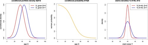
In Figure 1 (lhs) we give an explicit example for model (11(11) $(X,D)\sim f(x,d)=\frac{1}{2}\frac{1}{\sqrt{2\pi {\tau }^2}}\exp \{-\frac{1}{2{\tau }^2}{(x-x_d)}^2\},$(11) ). This plot shows the conditional Gaussian densities of X, given $D=d\in \{0,1\}$; we select $x_0=35$, age gap $\delta =10$ (providing $x_1=45$), and $\tau =10$. We can easily calculate the conditional probability of D = 0 (being woman), given age X, (14) $\mathbb{P}\left(D=0|X\right)=\frac{\exp \{-\frac{1}{2{\tau }^2}{(X-x_0)}^2\}}{\sum _{d\in \mathfrak{D}}\exp \{-\frac{1}{2{\tau }^2}{(X-x_d)}^2\}}\in (0,1).$(14) Figure 1 (middle) shows these conditional probabilities as a function of the age variable X = x. For small X we have likely a woman, D = 0, and for large X a man, D = 1. Figure 1 (rhs) shows the Gaussian densities of the claims Y at the given age X = 40 and for both genders D = 0, 1. The vertical dotted line shows the resulting means (13(13) $\mu (\mathit{X},\mathit{D})=\mu (\mathit{X})={\mu }^{\ast }(\mathit{X})=X.$(13) ). These means coincide for both genders D = 0, 1, and the protected attribute D only influences the width of the Gaussian densities, see (12(12) $Y{|}_{(\mathit{X},\mathit{D})}\sim \mathcal{N}(X,1+D).$(12) ).

We give some general remarks on Example 2.12.

Figure 1. (lhs) Conditional Gaussian densities $f(x|d)$ for $d\in \mathfrak{D}=\{0,1\}$; (middle) conditional probability $\mathbb{P}(D=0|X=x)$ as a function of $x\in \mathbb{R}$; (rhs) densities of claims Y for age X = 40 and genders D = 0, 1.

Remarks 2.13

• A crucial feature of Example 2.12 is that the non-protected covariates $\mathit{X}$ are sufficient to describe the mean of the response Y, and the protected attributes $\mathit{D}$ only impact higher moments of Y. Therefore, no material proxy discrimination arises in this example from using the unawareness price, because (13(13) $\mu (\mathit{X},\mathit{D})=\mu (\mathit{X})={\mu }^{\ast }(\mathit{X})=X.$(13) ) holds. From a practical point of view we may question such a model, but it has the advantage for the subsequent discussions that we do not need to rely on any type of proxy discrimination debiasing for stating the crucial points about group fairness and discrimination. We could modify (12(12) $Y{|}_{(\mathit{X},\mathit{D})}\sim \mathcal{N}(X,1+D).$(12) ) to include $\mathit{D}$ also in the first moment of Y and derive similar conclusions, but then we would first need to convince the reader that the DFIP ${\mu }^{\ast }(\mathit{X})$ is indeed the right way to correct for proxy discrimination.

• A situation where protected attributes $\mathit{D}$ only impact higher moments may arise in the case of a lack of historical data of a demographic group. This may lead to higher uncertainty, reflected in higher moments, but not the means. From an insurance pricing point of view, this manifests in higher risk loadings, which may then be subject to discrimination. Even though the use of risk loadings is not inconsistent with our Definitions 2.1 and 2.2, pricing functionals involving loadings are not discussed further in this paper. The situation where predictions for different demographic groups are subject to higher uncertainty finds parallels in the machine learning literature, where there is concern about poor performance of predictive models for populations that are under-represented in training samples, e.g. in the context of facial recognition see (Buolamwini & Gebru, 2018). The crucial point is whether such increased uncertainty has adverse impacts on these demographic groups, such as a higher likelihood of misidentification leading to systematic penalties, see, e.g. (Vallance, 2021).

We now present a variation of the previous example, where the dependence of $(\mathit{X},\mathit{D})$ leads to proxy discrimination, which requires correction in the sense of Equation (9(9) ${\mu }^{\ast }(\mathit{X},\mathbb{P}):=\sum _{\mathit{d}\in \mathfrak{D}}\mu (\mathit{X},\mathit{d},\mathbb{P}){\mathbb{P}}^{\ast }(\mathit{D}=\mathit{d}),$(9) ).

Example 2.14

Proxy discrimination and DFIP

We again assume two-dimensional covariates $(\mathit{X},\mathit{D})=(X,D)$ having the same mixture Gaussian distribution as in (11(11) $(X,D)\sim f(x,d)=\frac{1}{2}\frac{1}{\sqrt{2\pi {\tau }^2}}\exp \{-\frac{1}{2{\tau }^2}{(x-x_d)}^2\},$(11) ). For the response variable Y we now assume that conditionally, given $(\mathit{X},\mathit{D})$, (15) $Y{|}_{(\mathit{X},\mathit{D})}\sim \mathcal{N}(X+20(1-D){\mathbb{1}}_{X\in [20,40]}-10D,100).$(15) For Y representing health claims, the interpretation of this model is that female policyholders (D = 0) between ages 20 and 40 generate higher costs due to a potential pregnancy,¹ and male policyholders generally have lower costs.

The resulting best-estimate prices, illustrated in Figure 2 by the red and blue dotted lines, are given by $\mu (\mathit{X},\mathit{D})=\mathbb{E}[Y|\mathit{X},\mathit{D}]=X+20(1-D){\mathbb{1}}_{X\in [20,40]}-10D.$Hence, the above best-estimate prices have a sensitivity in $\mathit{D}$ and $\mathit{D}\perp ̸\perp \mathit{X}$, and Proposition 2.6 directly tells us that the corresponding unawareness prices are subject to proxy discrimination. Another crucial difference of these best-estimate prices compared to the ones in Example 2.12 is that we do not have monotonicity in $x\mapsto \mu (X=x,D=0)$ for women, e.g. there is not a unique age x that leads to the best-estimate price $\mu (x,0)=50$. This feature will become important later, when in Example 3.6 we apply output Optimal Transport methods to the same model.

We calculate the unawareness price $\mu (\mathit{X})=X+\frac{20\exp \{-\frac{1}{2{\tau }^2}{(X-x_0)}^2\}}{\sum _{d\in \mathfrak{D}}\exp \{-\frac{1}{2{\tau }^2}{(X-x_d)}^2\}}{\mathbb{1}}_{X\in [20,40]}-\frac{10\exp \{-\frac{1}{2{\tau }^2}{(X-x_1)}^2\}}{\sum _{d\in \mathfrak{D}}\exp \{-\frac{1}{2{\tau }^2}{(X-x_d)}^2\}},$where we have used (14(14) $\mathbb{P}\left(D=0|X\right)=\frac{\exp \{-\frac{1}{2{\tau }^2}{(X-x_0)}^2\}}{\sum _{d\in \mathfrak{D}}\exp \{-\frac{1}{2{\tau }^2}{(X-x_d)}^2\}}\in (0,1).$(14) ). This unawareness price is illustrated in orange colour in Figure 2. Not surprisingly, it closely follows the best-estimate prices for woman policyholders for small ages and men for large ages, because we can infer the gender D from the age X quite well, see Figure 1 (middle). Thus, except in the age range from 20 to 60, we almost charge the best-estimate price to the corresponding genders, except to a few ‘mis-allocated’ men at small ages and women at high ages. This is precisely proxy discrimination and, in our understanding, consistent with what is described in paragraph 5 of Section 2 of Maliszewska-Nienartowicz (2014), and can be interpreted as generating a disproportionate impact on (woman) policyholders.

Figure 2. Best-estimate, unawareness and discrimination-free insurance prices in Example 2.14.

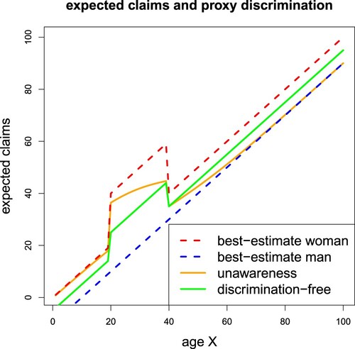
Subsequently, the DFIP, using the choice ${\mathbb{P}}^{\ast }(D=0)=1/2$, is shown in green colour in Figure 2 and reads as ${\mu }^{\ast }(\mathit{X})=X+10\cdot {\mathbb{1}}_{X\in [20,40]}-5.$The price ${\mu }^{\ast }(\mathit{X})$ exactly interpolates between the two best-estimate prices for women and men. As a result we have a cost reallocation between different ages which leads to a loss of predictive power and to cross-financing of claim costs within the portfolio.

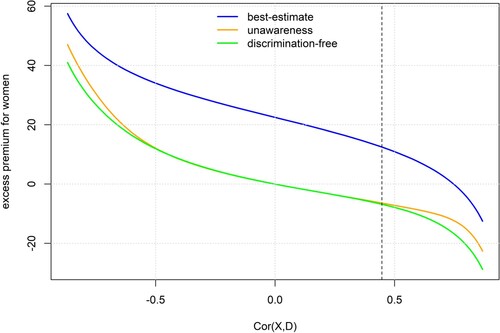
We now turn our attention to the differential outcomes for each gender, under each of the pricing mechanisms considered. Specifically, we calculate the ‘excess premium’ for women, as the difference of the average price for women (prices conditional on D = 0, minus the average price for men (prices conditional on D = 1). Furthermore, we consider how this excess premium varies in the correlation $\mathrm{Cor}(X,D)$, which we can control via the model parameter δ (age gap) and plot the results in Figure 3. We observe that, as correlation increases, there is a sharper distinction between older male and younger female policyholders, which, given the effect of age on claims, reduces the excess premium for women. Furthermore, as expected, the excess premium is reduced by switching from best-estimate (blue) to either unawareness prices (green) or DFIP (orange). Furthermore, for all correlation values, the excess premium for the unawareness price dominates that for the DFIP, since the proxying of gender by age (more pronounced for correlation close to $\pm 1$), increases prices for women. However, this does not mean that using the DFIP produces more equal outcomes for each gender. Specifically, for high correlation values we see that the excess premium for ${\mu }^{\ast }(X)$ is the highest in absolute value.

Figure 3. Average excess premium for women D = 0 compared to men D = 1, in Example 2.14, as a function of $\mathrm{Cor}(X,D)$. The dashed vertical line corresponds to the baseline scenario of $x_0=35,x_1=45$, $\mathrm{Cor}(X,D)=0.447$.

Finally, it is also of interest to establish how the different pricing functionals we consider perform as predictors of Y. Let Π be a random variable, representing the statistical behaviour under $\mathbb{P}$ of insurance prices derived by a given pricing functional. For example, if $\mu (\mathit{X})$ is the unawareness price, $\mathrm{\Pi }=\mu (\mathit{X})$. Then, the performance of the price Π as a predictor of Y can be measured by the mean squared error (MSE), given by $\mathbb{E}[(Y-\mathrm{\Pi }{)}^2]$. We also consider a potential bias by providing the average prediction $\mathbb{E}[\mathrm{\Pi }]$ of the prices, over the portfolio distribution. We calculate the resulting MSEs using Monte Carlo simulation with a pseudo-random sample of size 1 million. The results in Table 1 show the negative impact of deviating from the optimal predictors, based on $(\mathit{X},\mathit{D})$ and $\mathit{X}$, respectively. This is the price we pay for avoiding proxy discrimination with respect to the protected attributes $\mathit{D}$. Our pricing measure choice ${\mathbb{P}}^{\ast }(D=0)=\mathbb{P}(D=0)=1/2$ produces a bias as can be seem from the last column of Table 1.

2.3. Group fairness axioms

As discussed in Section 2.1, the property of avoiding proxy discrimination can be understood as an individual fairness property, in the sense that it requires that similar policyholders, in the sense specified by Definition 2.2, be treated similarly. This has implications on how the pricing functionals (9(9) ${\mu }^{\ast }(\mathit{X},\mathbb{P}):=\sum _{\mathit{d}\in \mathfrak{D}}\mu (\mathit{X},\mathit{d},\mathbb{P}){\mathbb{P}}^{\ast }(\mathit{D}=\mathit{d}),$(9) ) avoiding proxy discrimination are constructed, without exploiting the dependence structure of $\mathit{X}$ and $\mathit{D}$. On the other hand, as demonstrated in Example 2.14, Figure 3, addressing proxy discrimination does not consider at all the statistical properties of DFIPs; for example, for $\mathit{d}\ne {\mathit{d}}^{\prime }$, it will generally hold that (16) $\mathbb{E}[{\mu }^{\ast }(\mathit{X})\mid \mathit{D}=\mathit{d}]\ne \mathbb{E}[{\mu }^{\ast }(\mathit{X})\mid \mathit{D}={\mathit{d}}^{\prime }],$(16) such that different demographic groups, on average, are charged different premiums.

Table 1. MSEs and average prediction of the different prices in Example 2.14.

price Π	MSE	average price
Best-estimate price $\mu (\mathit{X},\mathit{D})$	100.00	41.25
Unawareness price $\mu (\mathit{X})$	197.20	41.25
DFIP ${\mu }^{\ast }(\mathit{X})$ with ${\mathbb{P}}^{\ast }(D=0)=0.50$	217.66	39.63

To address concerns about the implications of using any pricing method for the outcomes for different demographic groups, we need to consider the resulting prices as random variables. As an example, the right-hand side of (16(16) $\mathbb{E}[{\mu }^{\ast }(\mathit{X})\mid \mathit{D}=\mathit{d}]\ne \mathbb{E}[{\mu }^{\ast }(\mathit{X})\mid \mathit{D}={\mathit{d}}^{\prime }],$(16) ) uses the random selection of an insurance policy $\mathit{X}$ and its related price ${\mu }^{\ast }(\mathit{X})$, respectively, from the insurance portfolio, conditioned on selecting an insurance policy with protected attributes $\mathit{D}=\mathit{d}$. Throughout this section, we denote the prices in an insurance portfolio by the random variable Π. We may interpret $\mathrm{\Pi }(\omega )$ as the price for a policyholder with profile $(\mathit{x},\mathit{d})=(\mathit{X},\mathit{D})(\omega )$, $\omega \in \mathrm{\Omega }$. If π is a pricing functional, then we can set $\mathrm{\Pi }=\pi (\mathit{X},\mathbb{P})$, such that Π is $\sigma (\mathit{X})$-measurable; note however that the definitions of the group fairness properties below do not rely on such a measurability condition on Π.

We now introduce the three most popular group fairness properties in the machine learning literature, which are essentially properties of the joint distribution of $(\mathrm{\Pi },Y,\mathit{D})$. The properties we consider here are demographic parity, equalized odds and predictive parity; we refer to Barocas et al. (2019), Xin and Huang (2021) and Charpentier (2022). In the next section, we show that the DFIP of Example 2.12, given in Equation (13(13) $\mu (\mathit{X},\mathit{D})=\mu (\mathit{X})={\mu }^{\ast }(\mathit{X})=X.$(13) ), violates all three of these group fairness axioms. These three notations of group fairness are collected next definition.

Definition 2.15

The prices Π, in the context of portfolio distribution $\mathbb{P}$, satisfy:

1. Demographic parity, if Π and $\mathit{D}$ are independent under $\mathbb{P}$, implying that $\mathbb{P}$-a.s., (17) $\mathbb{P}\left(\mathrm{\Pi }\le m|\mathit{D}\right)=\mathbb{P}(\mathrm{\Pi }\le m)\mathrm{for}\mathrm{all}m\in \mathbb{R}.$(17)

2. Equalized odds, if Π and $\mathit{D}$ are conditionally independent under $\mathbb{P}$, given Y, implying that $\mathbb{P}$-a.s., (18) $\mathbb{P}(\mathrm{\Pi }\le m|Y,\mathit{D})=\mathbb{P}\left(\mathrm{\Pi }\le m|Y\right)\mathrm{for}\mathrm{all}m\in \mathbb{R}.$(18)

3. Predictive parity, if Y and $\mathit{D}$ are conditionally independent under $\mathbb{P}$, given Π, implying that $\mathbb{P}$-a.s., (19) $\mathbb{P}(Y\le y|\mathrm{\Pi },\mathit{D})=\mathbb{P}\left(Y\le y|\mathrm{\Pi }\right)\mathrm{for}\mathrm{all}y\in \mathbb{R}.$(19)

We comment on each of the three group fairness notions of Definition 2.15 below, focussing on the conditions needed for pricing mechanisms to satisfy them and whether they can be realistically expected to hold within insurance portfolios. We note that in the fairness and machine learning literature, see, e.g. (Barocas et al., 2019), the equalized odds and predictive parity properties are primarily used for binary responses, which is of less relevance for actuarial pricing applications.

Remarks 2.16

• Demographic parity (Agarwal et al., 2019; also: statistical parity, independence axiom) is the simplest notion to interpret. If Π satisfies demographic parity, this directly implies $\mathbb{E}[\mathrm{\Pi }\mid \mathit{D}=\mathit{d}]=\mathbb{E}[\mathrm{\Pi }\mid \mathit{D}={\mathit{d}}^{\prime }]=\mathbb{E}[\mathrm{\Pi }],$for all $\mathit{d},{\mathit{d}}^{\prime }\in \mathfrak{D}$, which can be contrasted with (16(16) $\mathbb{E}[{\mu }^{\ast }(\mathit{X})\mid \mathit{D}=\mathit{d}]\ne \mathbb{E}[{\mu }^{\ast }(\mathit{X})\mid \mathit{D}={\mathit{d}}^{\prime }],$(16) ). Hence, policyholders in different protected demographic groups are on average charged the same premium. If the prices Π are $\sigma (\mathit{X})$-measurable, then a sufficient (but not necessary) condition for Π to satisfy demographic parity is that $\mathit{X}$ and $\mathit{D}$ are independent. In practice that would mean that the insurance portfolio is composed in a way such that the conditional distribution of the non-protected covariates $\mathit{X}$, given $\mathit{D}$, is the same for all demographic groups $\mathit{D}=\mathit{d}\in \mathfrak{D}$. This condition is hard to achieve in a portfolio, even by design. If $\mathit{D}$ describes gender, there may be general insurance products where this is feasible (property insurance). However, e.g. in commercial accident insurance this may not be possible, because the genders are represented with different frequencies in different job profiles, which may make it impossible to compose a portfolio such that the selected jobs have the same distribution for both genders.

  Moreover, we may have two different insurance companies with portfolio distributions ${\mathbb{P}}_1$ and ${\mathbb{P}}_2$ that only differ in the dependence structure, and which apply the same pricing mechanism Π to the same insurance product Y. It may happen, under specific assumptions on ${\mathbb{P}}_1$ and ${\mathbb{P}}_2$, that one company satisfies demographic parity and the other one not. This seems difficult to explain and accept.

• Equalized odds (Hardt et al., 2016; also: disparate mistreatment, separation axiom) implies that within groups of policyholders that produce the same level claims, the prices are independent of protected attributes. In general, independence between $\mathit{X}$ and $\mathit{D}$ is not sufficient to receive equalized odds for a $\sigma (\mathit{X})$-measurable predictor Π. It is generally difficult for prices to satisfy equalized odds, as – particularly in the non-binary response case of insurance portfolios – this property depends on the structure of the predictors. Specifically, there are scenarios where conditional independence is impossible, as when $\mathit{D}$ and Y jointly fully determine $\mathit{X}$ (and hence a $\sigma (\mathit{X})$-measurable price Π), e.g. in the case of sex-specific claims that only occur within disjoint age groups. The key limitation is that, while the portfolio composition $\mathbb{P}(\mathit{X},\mathit{D})$ is to an extent in the hands of the insurers, risk factor design is not always possible through insurance cover design.

• The notion of predictive parity (Barocas et al., 2019; also: sufficiency axiom) can be motivated by the definition of a sufficient statistic in statistical estimation theory. We can interpret $\mathfrak{P}=\{{\mathbb{P}}_{\mathit{d}}(Y\in \cdot ):=\mathbb{P}(Y\in \cdot |\mathit{D}=\mathit{d});\mathit{d}\in \mathfrak{D}\}$ as a family of distributions of Y being parameterized by $\mathit{d}\in \mathfrak{D}$. If prices Π are $\sigma (\mathit{X})$-measurable and we interpret statistically Π as a predictor of Y, then Π is called sufficient for $\mathfrak{P}$ if (19(19) $\mathbb{P}(Y\le y|\mathrm{\Pi },\mathit{D})=\mathbb{P}\left(Y\le y|\mathrm{\Pi }\right)\mathrm{for}\mathrm{all}y\in \mathbb{R}.$(19) ) holds. Essentially, this means that Π carries all the necessary information needed to predict Y, such that explicit knowledge of $\mathit{D}=\mathit{d}$ becomes redundant. However, such an assumption seems unrealistic in an insurance pricing context, because there is hardly any example in which all relevant information for claims prediction can be fully condensed into a single predictor Π. Note that even in the case that $(Y,\mathit{D})$ are conditionally independent given $\mathit{X}$, it does not follow that (19(19) $\mathbb{P}(Y\le y|\mathrm{\Pi },\mathit{D})=\mathbb{P}\left(Y\le y|\mathrm{\Pi }\right)\mathrm{for}\mathrm{all}y\in \mathbb{R}.$(19) ) holds true.

Regardless of the actuarial relevance of the fairness notions of Definition 2.15 it is clear that rather special conditions are needed in order for all of them to hold jointly. The following proposition provides such a sufficient condition:

Proposition 2.17

Assume that the prices Π, in the context of portfolio distribution $\mathbb{P}$, satisfy $(Y,\mathrm{\Pi })\perp \perp \mathit{D}.$The prices Π then satisfies fairness notions (i)–(iii) from Definition 2.15.

The proof is given in Appendix 1.

2.4. Discrimination-free vs. fair insurance prices

In Example 2.14 and Section 2.3, we discussed how avoiding proxy discrimination and achieving outcomes across demographic groups that satisfy a group fairness criterion are rather different requirements. We now formalize this insight via the following two propositions.

Proposition 2.18

Consider the pricing functional π and the respective prices $\mathrm{\Pi }=\pi (\mathit{X},\mathbb{P})$. If π avoids proxy discrimination, it is not implied that Π satisfies any of demographic parity, equalized odds or predictive parity.

Proposition 2.19

Consider the pricing functional π and the respective prices $\mathrm{\Pi }=\pi (\mathit{X},\mathbb{P})$. If Π satisfies demographic parity, it is not implied that π avoids proxy discrimination.

A particular implication of Propositions 2.18 and 2.19 is that avoiding proxy discrimination is generally not a stronger requirement than avoiding group fairness notions (and vice versa). As both propositions are negative results, they can be proved by counter-examples. For Proposition 2.18 this is Example 2.12. In that example, the DFIP produces violations of all three group fairness properties considered here. The required derivations to show this are somewhat laborious and, thus, are delegated to Appendix 1. As the DFIP in that example is identical to the unawareness price, one cannot claim that these violations are specific to the construction of ${\mu }^{\ast }(\mathit{X})$. The crucial feature of Example 2.12 is that the non-protected covariates $\mathit{X}$ are sufficient for describing the conditional expectation of the response Y, but they are not sufficient to describe the full conditional distribution of Y, given $(\mathit{X},\mathit{D})$.

To prove Proposition 2.19, a suitable counter-example is given in Example 2.20, below; here we provide a situation where the unawareness price does not materially avoid proxy discrimination, while at the same time it satisfies demographic parity. Furthermore, in an additional Example 2.21, below, we offer a situation which produces prices that satisfy all of demographic parity, equalized odds and predictive parity, but which directly discriminate, in the sense that they are explicit functions of protected attributes $\mathit{D}$. Of course, if such direct discrimination takes place, one cannot meaningfully say that proxy discrimination is avoided.

Remark that in the following examples, we consider a real-valued Gaussian distributed protected attribute $\mathit{D}=D$. This is in contrast to assuming that $\mathfrak{D}$ is finite, see Section 2.1. The reason for this different choice is a computational one because in a multivariate Gaussian setting all quantities of interest can be calculated explicitly. In the examples the protected attribute $\mathit{D}=D$ and the non-protected covariates will be positively correlated, which allows inferring one from the other.

Example 2.20

Demographically fair prices that produce proxy discrimination

We choose three-dimensional Gaussian covariates (20) $(\mathit{X},\mathit{D})=(X_1,X_2,D)\sim \mathcal{N}(\left(\begin{array}{c}0\\ 0\\ 0\end{array}\right),\left(\begin{array}{ccc}2& 1& 1\\ 1& 2& 1\\ 1& 1& 2\end{array}\right)).$(20) For the response variable we assume ${Y|}_{(\mathit{X},\mathit{D})}\sim \mathcal{N}(2X_1-3D,1).$This gives us the best-estimate price (21) $\mu (\mathit{X},\mathit{D})=2X_1-3D.$(21) A standard result on multivariate Gaussian random variables tells us, see, e.g. Corollary 4.4 in Wüthrich and Merz (2015), ${D|}_{\mathit{X}}\sim \mathcal{N}(\frac{X_1+X_2}{3},\frac{4}{3}).$This allows us to calculate the unawareness price by (22) $\mathrm{\Pi }:=\mu (\mathit{X})=\mathbb{E}\left[\mu (\mathit{X},\mathit{D})|\mathit{X}\right]=2X_1-\mathbb{E}\left[3D|\mathit{X}\right]=X_1-X_2,$(22) which is different to the DFIP, ${\mu }^{\ast }(\mathit{X})=2X_1-\mathbb{E}[3D]=2X_1$. We know that the unawareness price in general does not avoid proxy discrimination. Since the best-estimate price has a sensitivity in D and because there is dependence between $\mathit{X}$ and D, proxy discrimination is material; recall Proposition 2.6. In fact, not considering non-protected covariates $\mathit{X}$ leads to a prediction of the protected attribute D of $\mathbb{E}[D]=0$. Since $\mathit{X}$ and D are positively correlated, we can (partly) infer D from $\mathit{X}$ by using the (informed) prediction $\mathbb{E}[D|\mathit{X}]=(X_1+X_2)/3$, e.g. if both $X_1$ and $X_2$ take positive values, we get a positive predicted value for D, given $\mathit{X}$.

The random vector $(X_1-X_2,D)$ is two-dimensional Gaussian with independent components because $\mathrm{Cov}(X_1-X_2,D)=\mathrm{Cov}(X_1,D)-\mathrm{Cov}(X_2,D)=0.$This implies that the unawareness price $\mathrm{\Pi }=\mu (\mathit{X})=X_1-X_2$ is independent of D, hence, it satisfies demographic parity. This also proves Proposition 2.19.

We now give an example that satisfies all three group fairness criteria of demographic parity, equalized odds and predictive parity, but at the same time directly discriminates.

Example 2.21

Group fair prices that directly discriminate

Assume the non-protected covariates $\mathit{X}=X$ and the protected attribute $\mathit{D}=D$ are real-valued. We choose a three-dimensional Gaussian distribution $(Y,X,D{)}^{\mathrm{\top }}\sim \mathcal{N}(\left(\begin{array}{c}0\\ 0\\ 0\end{array}\right),\left(\begin{array}{ccc}1& \rho & 0\\ \rho & 2& 1\\ 0& 1& 1\end{array}\right)),$with fixed covariance parameter $\rho \in (0,1)$. The best-estimate is given by (23) $\begin{array}{rl}\mu (X,D)& =\mathbb{E}[Y|X,D]=0+(\rho ,0){\left(\begin{array}{cc}2& 1\\ 1& 1\end{array}\right)}^{-1}(\left(\begin{array}{c}X\\ D\end{array}\right)-\left(\begin{array}{c}0\\ 0\end{array}\right))\\ & =(\rho ,0)\left(\begin{array}{cc}1& -1\\ -1& 2\end{array}\right)\left(\begin{array}{c}X\\ D\end{array}\right)=\rho (X-D),\end{array}$(23) this uses again Corollary 4.4 of Wüthrich and Merz (2015). This best-estimate price directly discriminates because it uses D as an input. We now show that $\mu (X,D)$ satisfies all three notions of group fairness. For this, we derive the joint distribution of $(Y,\mu (X,D),D)$. Note that $\left(\begin{array}{c}Y\\ \mu (X,D)\\ D\end{array}\right)=B\left(\begin{array}{c}Y\\ X\\ D\end{array}\right),\mathrm{where}B=\left(\begin{array}{ccc}1& 0& 0\\ 0& \rho & -\rho \\ 0& 0& 1\end{array}\right).$Hence, $\left(\begin{array}{c}Y\\ \mu (X,D)\\ D\end{array}\right)\sim \mathcal{N}(\left(\begin{array}{c}0\\ 0\\ 0\end{array}\right),B\left(\begin{array}{ccc}1& \rho & 0\\ \rho & 2& 1\\ 0& 1& 1\end{array}\right)B^{\mathrm{\top }})\stackrel{(\mathrm{d})}{=}\mathcal{N}(\left(\begin{array}{c}0\\ 0\\ 0\end{array}\right),\left(\begin{array}{ccc}1& {\rho }^2& 0\\ {\rho }^2& {\rho }^2& 0\\ 0& 0& 1\end{array}\right)).$This shows that $(Y,\mu (X,D))$ and D are independent, which is precisely the sufficient condition presented in Proposition 2.17. As a result, all three group fairness axioms above are fulfilled for the best-estimate price $\mathrm{\Pi }=\mu (X,D)$. On the other hand, this best-estimate directly discriminates as can be seen from (23(23) $\begin{array}{rl}\mu (X,D)& =\mathbb{E}[Y|X,D]=0+(\rho ,0){\left(\begin{array}{cc}2& 1\\ 1& 1\end{array}\right)}^{-1}(\left(\begin{array}{c}X\\ D\end{array}\right)-\left(\begin{array}{c}0\\ 0\end{array}\right))\\ & =(\rho ,0)\left(\begin{array}{cc}1& -1\\ -1& 2\end{array}\right)\left(\begin{array}{c}X\\ D\end{array}\right)=\rho (X-D),\end{array}$(23) ).

We now give some additional remarks on Propositions 2.18 and 2.19 and Example 2.21.

Remarks 2.22

• Propositions 2.18 and 2.19 indicate that avoiding proxy discrimination and satisfying group fairness are rather different concepts, and, in general, one does not imply the other. For this reason, satisfying simultaneously both is more restrictive than just complying with one of them – and sometimes even impossible if one wants to have a non-trivial predictor. Currently, many regulators focus on proxy discrimination, though corresponding legislation leaves room for interpretation. Therefore, constraining pricing models with group fairness criteria does not seem to solve this particular regulatory problem.

• Proxy discrimination is caused by two factors that need to hold simultaneously, namely, (1) there needs to be a dependence between the non-protected covariates $\mathit{X}$ and the protected attributes $\mathit{D}$, and (2) there needs to be a sensitivity of the best-estimate price $\mu (\mathit{X},\mathit{D})$ in $\mathit{D}$, recall Proposition 2.6. These conditions (or the lack of them) do not tell us anything about the dependence structure between a DFIP ${\mu }^{\ast }(\mathit{X})$ and $\mathit{D}$. In general, ${\mu }^{\ast }(\mathit{X})$ and $\mathit{D}$ are correlated, namely, observe that the dependence structure between $\mathit{X}$ and $\mathit{D}$ is completely irrelevant for the calculation of the DFIP from (9(9) ${\mu }^{\ast }(\mathit{X},\mathbb{P}):=\sum _{\mathit{d}\in \mathfrak{D}}\mu (\mathit{X},\mathit{d},\mathbb{P}){\mathbb{P}}^{\ast }(\mathit{D}=\mathit{d}),$(9) ). Therefore, we can always find a portfolio distribution $\mathbb{P}(\mathit{X},\mathit{D})$ under which the price ${\mu }^{\ast }(\mathit{X})$ and the protected attributes $\mathit{D}$ are dependent, unless ${\mu }^{\ast }(\mathit{X})$ does not depend on $\mathit{X}$.

• Focusing on the example of demographic parity fairness, this notion solely relates to the independence of the resulting prices Π and protected attributes $\mathit{D}$. Let $\mathrm{\Pi }=\pi (\mathit{X})$, such that prices are $\sigma (\mathit{X})$-measurable. If this price Π satisfies demographic parity, then $\mathit{X}\mapsto \pi (\mathit{X})$ can be interpreted as a projection that only extracts the information from $\mathit{X}$ that is orthogonal to/independent of $\mathit{D}$; this is similar to the linear adversarial concept erasure of Ravfogel et al. (2020, 2022); see also Example 2.20. That Π becomes independent of $\mathit{D}$ is a specific property of the pricing functional $\mathit{X}\mapsto \pi (\mathit{X})$ in relation to $\mathit{D}$, but this does not account for the full dependence structure in $\mathbb{P}(\mathit{X},\mathit{D})$ nor for the properties in the best-estimate price $\mu (\mathit{X},\mathit{D})$. Therefore, in general, demographic parity does not constitute evidence regarding proxy discrimination.

  If we wanted all participants in an insurance market to comply with demographic parity, we would need to choose projections $\mathit{X}\mapsto \pi (\mathit{X})$ that vary from company to company because they all have different portfolio distributions $\mathbb{P}(\mathit{X},\mathit{D})$. As a result, every company would consider non-protected covariates in a different way. This would be difficult to explain to customers and may be impossible to regulate; we also refer to the first item of Remark 2.16 (last paragraph). Therefore, stronger assumptions are typically explored, like aiming at full independence between $\mathit{X}$ and $\mathit{D}$, see Section 3.2, below.

• A crucial feature of Example 2.20 is that independence between $\mathit{X}$ and $\mathit{D}$ is a sufficient condition to have demographic parity fairness, but not a necessary one. This is used in an essential way, namely, $\mathit{X}$ and $\mathit{D}$ are dependent, but the projection $\mathit{X}\mapsto \mu (\mathit{X})$ only extracts a part of information from $\mathit{X}$ that is independent of $\mathit{D}$. Example 2.21 goes even further, by demonstrating a situation where a price that satisfies demographic parity, equalized odds and predictive parity directly discriminates.

• Examples 2.20 and 2.21 use multivariate Gaussian distributions, since these make all relevant calculations straightforward. This is not a limitation, as similar examples can be constructed with discrete protected attributes $\mathit{D}$. However, such discrete examples typically become more demanding computationally, making them less transparent in terms of exposition. Note that the counter-examples are only used to prove the negative results of Propositions 2.18 and 2.19 and this is mathematically correct regardless of whether these counter-example are realistic or not. If we restrict our attention to demographic parity and proxy discrimination it is easy to construct non-Gaussian counter-examples verifying the statements (in this restricted sense) of Propositions 2.18 and 2.19. This is done in Appendix 2.

3. Achieving demographic parity by optimal transport methods

3.1. Rationale

In Section 2, we formalized our view of direct and proxy discrimination, and we discussed pricing functionals that avoid them. Furthermore, we established that group fairness concepts are not generally consistent with the requirement of avoiding direct and proxy discrimination; essentially they provide answers to different problems. Next, we focus on methods to create pricing functionals that satisfy group fairness and discuss their implications for both direct and proxy discrimination.

In this section, we will specifically focus on demographic parity as a group fairness concept. The reason for this is three-fold:

1. Let us take as a starting point the need to avoid proxy discrimination. We have noted that in the special case where $\mathit{X}$ and $\mathit{D}$ are independent, the unawareness price is identical to the DFIP, henceforth, using the unawareness price would not introduce material proxy discrimination. This motivates the question: if $\mathit{X}$ and $\mathit{D}$ are not independent, is there a way to make them so? We will show in this section how optimal transport (OT) methods can help to achieve precisely that. But note also that independence of $\mathit{X}$ and $\mathit{D}$ implies the independence of any $\sigma (\mathit{X})$-measurable price from the protected attributes $\mathit{D}$ and, hence, demographic parity. This means that, despite the conflict between the two concepts we already discussed, there is further scope to interrogating their relationship.

2. Demographic parity is a much simpler concept to explain to stakeholders, including policyholders. While no form of group fairness is mandated by regulators, insurers will remain sensitive to reputational risk, which itself derives from those violations of group fairness that are most easily monitored; see, e.g. the Citizens Advice report (Cook et al., 2022). We do not envisage that insurance companies will or indeed should aim to satisfy demographic parity and, in fact, we argue against this in the sequel. But companies may be motivated to monitor demographic disparities and in some cases partially smooth out these effects, e.g. using the methods of Grari et al. (2022).

3. As argued in Remarks 2.16, demographic parity may sometimes be achieved by a careful selection of the policyholders in the portfolio (aiming to have $\mathit{D}$ independent of $\mathit{X}$ under $\mathbb{P}$) or by introducing direct discrimination. The latter approach is reflected in Example 2.21 and, in a sense, underlies the methods of the current section (which can be criticized on precisely that basis). Therefore, verifying/satisfying demographic parity is often easier than equalized odds and predictive parity. In particular, it requires less insurance policy engineering.

In the rest of this Section, we will use the theory of optimal transport (OT) for input pre-processing and output post-processing, see (Chiappa et al., 2020; del Barrio et al., 2019), with the aim of achieving demographic parity. By using these techniques it will also be possible to relate the price deformations needed in order to achieve demographic parity to the construction of DFIPs. For both types of OT, independence of prices from protected attributes is achieved by a $\mathit{D}$-dependent transformation of the non-protected covariates $\mathit{X}$. An important difference between input pre-processing and model post-processing is that the former transforms the inputs $\mathit{X}\mapsto {\mathit{X}}_{+}$, and retains the dimension of the original non-protected covariates $\mathit{X}$. In fact, up to technical conditions (continuity), the OT input transformation $\mathit{X}\mapsto {\mathit{X}}_{+}$ is one-to-one (for given $\mathit{D}$) which allows us to reconstruct the original features $\mathit{X}$ from the pre-processed ones ${\mathit{X}}_{+}$. Model post-processing, using an OT map, transforms the (one-dimensional) regression output $\mu (\mathit{X},\mathit{D})\mapsto {\mu }_{+}$, by making ${\mu }_{+}$ independent of the protected attributes $\mathit{D}$. We have already seen in Example 2.21 a situation where the best-estimate price $\mu (\mathit{X},\mathit{D})=\rho (X-D)$ is independent of $\mathit{D}=D$, hence satisfies demographic parity. In that example the best-estimate price can be identified with ${\mu }_{+}$ and the OT output map is the identity map.

3.2. Input (data) pre-processing

A sufficient way to make an insurance price satisfy demographic parity is to pre-process the non-protected covariates $\mathit{X}\mapsto {\mathit{X}}_{+}$ such that the transformed version ${\mathit{X}}_{+}$ becomes independent of the protected attributes $\mathit{D}$ under $\mathbb{P}$. First, we emphasize that this pre-processing is only performed on the input data $\mathit{X}$ (and using $\mathit{D}$), but it does not consider the response Y. Second, independence between ${\mathit{X}}_{+}$ and $\mathit{D}$ is a sufficient condition for satisfying demographic parity with respect to $({\mathit{X}}_{+},\mathit{D})$, but not a necessary one, see Example 2.20.

One method of input pre-processing is to apply an OT map to obtain a covariate distribution that is independent of the protected attributes; for references see (Chiappa et al., 2020; del Barrio et al., 2019). More specifically, for given $\mathit{d}\in \mathfrak{D}$, we change the conditional distribution $F_{\mathit{d}}$ (24) ${\mathit{X}}_{\mathit{d}}:={\mathit{X}|}_{\{\mathit{D}=\mathit{d}\}}\sim F_{\mathit{d}}(\mathit{x}):=F(\mathit{x}|\mathit{D}=\mathit{d}),$(24) to an unconditional distribution $F_{+}$ for the non-protected covariates (25) ${{\mathit{X}}_{+}|}_{\mathit{D}}\sim F_{+}\left(\mathit{x}\right),$(25) meaning that the transformed covariates ${\mathit{X}}_{+}\sim F_{+}$ are independent of $\mathit{D}$. Intuitively, to minimally change the predictive power by this transformation from (24(24) ${\mathit{X}}_{\mathit{d}}:={\mathit{X}|}_{\{\mathit{D}=\mathit{d}\}}\sim F_{\mathit{d}}(\mathit{x}):=F(\mathit{x}|\mathit{D}=\mathit{d}),$(24) ) to (25(25) ${{\mathit{X}}_{+}|}_{\mathit{D}}\sim F_{+}\left(\mathit{x}\right),$(25) ), the unconditional distribution $F_{+}$ should be as similar as possible to the conditional ones $F_{\mathit{d}}$, for all $\mathit{d}\in \mathfrak{D}$; we come back to this in Remark 3.4, below. In this approach, the covariates $\mathit{X}$ and ${\mathit{X}}_{+}$ preserve their meanings because they live on the same covariate space, but the OT map locally perturbs the original covariate values ${\mathit{X}}_{\mathit{d}}\mapsto \mathit{X}$, based on $\mathit{D}=\mathit{d}$.

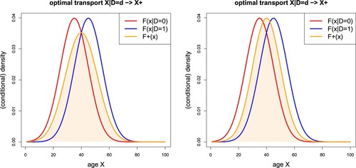
We revisit Examples 2.12 and 2.14 illustrated in Figure 1, and we give two different proposals for $F_{+}$ in Figure 4. The plot on the left hand side shows the average density $f_{+}$ of the two Gaussian densities $f_d(x):=f(x|D=d)$, given $D=d\in \{0,1\}$, i.e. we have a Gaussian mixture for $f_{+}$ on the left hand side of Figure 4. The plot on the right hand side shows the Gaussian density for $f_{+}$, that averages the means $x_0$ and $x_1$; we also refer to (31(31) $F_{+}(x)=\frac{1}{2}\mathrm{\Phi }\left(\frac{x-x_0}{\tau }\right)+\frac{1}{2}\mathrm{\Phi }\left(\frac{x-x_1}{\tau }\right),$(31) )–(32(32) $F_{+}(x)=\frac{1}{2}\mathrm{\Phi }\left(\frac{x-(x_0+x_1)/2}{\tau }\right).$(32) ), below. For the moment, it is unclear which of the two choices for $F_{+}$ gives a better predictive model for Y; we also refer to Remark 3.4, below.

Assume we have selected an unconditional distribution $F_{+}$ to approximate $F_{\mathit{d}}$, $\mathit{d}\in \mathfrak{D}$, and we would like to optimally transform the random variable ${\mathit{X}}_{\mathit{d}}$ to its unconditional counterpart ${\mathit{X}}_{+}$. This is precisely where OT comes into play. Choose a distance function ϱ on the covariate space. The (2-)Wasserstein distance between $F_{\mathit{d}}$ and $F_{+}$ w.r.t. ϱ is defined by (26) ${\mathcal{W}}_2(F_{\mathit{d}},F_{+}):={(\underset{{\pi }_{\mathit{d}}\in {\mathcal{P}}_{\mathit{d}}}{inf}\int \varrho (\mathit{x},{\mathit{x}}_{+}{)}^2\mathrm{d}{\pi }_{\mathit{d}}(\mathit{x},{\mathit{x}}_{+}))}^{1/2},$(26) where ${\mathcal{P}}_{\mathit{d}}$ is the set of all joint probability measures having marginals $F_{\mathit{d}}$ and $F_{+}$, respectively. The Wasserstein distance (26(26) ${\mathcal{W}}_2(F_{\mathit{d}},F_{+}):={(\underset{{\pi }_{\mathit{d}}\in {\mathcal{P}}_{\mathit{d}}}{inf}\int \varrho (\mathit{x},{\mathit{x}}_{+}{)}^2\mathrm{d}{\pi }_{\mathit{d}}(\mathit{x},{\mathit{x}}_{+}))}^{1/2},$(26) ) measures the difference between the two probability distributions $F_{\mathit{d}}$ and $F_{+}$ by optimally coupling them. Colloquially speaking, this optimal coupling means that we try to find the (optimal) transformation $T_{\mathit{d}}:{\mathit{X}}_{\mathit{d}}\mapsto {\mathit{X}}_{+}$ such that we can perform this change of distribution at a minimal effort;² this optimal transformation $T_{\mathit{d}}$ is called an OT map or a push forward. Under additional technical assumptions, determining the OT map $T_{\mathit{d}}:{\mathit{X}}_{\mathit{d}}\mapsto {\mathit{X}}_{+}$ is equivalent to finding the optimal coupling ${\pi }_{\mathit{d}}\in {\mathcal{P}}_{\mathit{d}}$.

Figure 4. Example 2.14, revisited: conditional densities $f_d(x)=f(x|D=d)$, for $d\in \{0,1\}$, and two different choices for $f_{+}(x)$, $x\in \mathbb{R}$; for a formal definition we refer to (31(31) $F_{+}(x)=\frac{1}{2}\mathrm{\Phi }\left(\frac{x-x_0}{\tau }\right)+\frac{1}{2}\mathrm{\Phi }\left(\frac{x-x_1}{\tau }\right),$(31) )–(32(32) $F_{+}(x)=\frac{1}{2}\mathrm{\Phi }\left(\frac{x-(x_0+x_1)/2}{\tau }\right).$(32) ).

Remarks 3.1

• The input OT approach can also be thought of in relation to context-sensitive covariates. For example, the European Commission (European Commission, 2012), footnote 1 to Article 2.2(14) – life and health underwriting – mentions the waist-to-hip ratio as a non-protected (useful) context-sensitive covariate for health prediction. Note that the waist-to-hip ratio is gender-, age- and race- dependent. Furthermore the impact of the waist-to-hip ratio on predictions of health outcomes depends specifically on factors like gender, age, and race, that is, the same value should be interpreted differently depending on the demographic group the policyholder belongs to. This means that a $\mathit{D}$-dependent transformation of the waist-to-hip ratio is desirable to achieve consistency.

  Applying an OT map will modify the waist-to-hip ratio such that it has the same distribution for both genders, which can then be treated coherently as an input to a predictive model. However, this does not mean that the transformed variable will reflect health impacts in a demographic-group-appropriate way, if the OT map produces a transformation specifically with the aim of removing dependence between $\mathit{X}$ and $\mathit{D}$ and, therefore, reflects the rather arbitrary dependence of those features in a particular portfolio. This also means that care should be taken more generally when considering OT-transformed covariates ${\mathit{X}}_{+}$, since their interpretation may not be straightforward. Still, if a transport map is derived from a population distribution of $(\mathit{X},\mathit{D})$ (e.g. of policyholders across a market), then demographic parity is expected to hold across the market (rather than on individual portfolios), and the transformed variables ${\mathit{X}}_{+}$ can be interpreted as $\mathit{D}$-agnostic versions of features $\mathit{X}$.

• In many situations the OT map $T_{\mathit{d}}:{\mathit{X}}_{\mathit{d}}\mapsto {\mathit{X}}_{+}$, $\mathit{d}\in \mathfrak{D}$, can be explicitly calculated, e.g. in the discrete covariate case it requires solving a linear program (LP); see (Cuturi & Doucet, 2014). The only difficulty in this discrete case is a computational one. Furthermore, the OT map is deterministic for continuous distributions, while in the case of discrete distributions we generally have a random OT map, see also (29(29) $V:=F_{\mathit{d}}(X_{-})+U(F_{\mathit{d}}(X_{-})-F_{\mathit{d}}(X)),$(29) ) below.

• The Wasserstein distance (26(26) ${\mathcal{W}}_2(F_{\mathit{d}},F_{+}):={(\underset{{\pi }_{\mathit{d}}\in {\mathcal{P}}_{\mathit{d}}}{inf}\int \varrho (\mathit{x},{\mathit{x}}_{+}{)}^2\mathrm{d}{\pi }_{\mathit{d}}(\mathit{x},{\mathit{x}}_{+}))}^{1/2},$(26) ) can also be defined for categorical covariates. The main difficulty in that case is that one needs to have a suitable distance function ϱ that captures the distance between categorical levels in a meaningful way.

• In general, this OT map should be understood as a local transformation of the covariate space, so that the main structure remains preserved, but the local assignments are perturbed differently for different realizations of $\mathit{D}$. In that, the non-protected covariates ${\mathit{X}}_{\mathit{d}}$ and ${\mathit{X}}_{+}$ keep their original interpretation, e.g. age of policyholder, but through a local perturbation some policyholders receive a slightly smaller or bigger age to make their distributions identical for all $\mathit{D}=\mathit{d}$, $\mathit{d}\in \mathfrak{D}$; note that these perturbations do not use the response Y, i.e. it is a pure input data transformation.

• Assume we have a (one-dimensional) real-valued non-protected covariate $\mathit{x}=x\in \mathbb{R}$ and we choose the Euclidean distance for ϱ. The dual formulation of the Wasserstein distance (26(26) ${\mathcal{W}}_2(F_{\mathit{d}},F_{+}):={(\underset{{\pi }_{\mathit{d}}\in {\mathcal{P}}_{\mathit{d}}}{inf}\int \varrho (\mathit{x},{\mathit{x}}_{+}{)}^2\mathrm{d}{\pi }_{\mathit{d}}(\mathit{x},{\mathit{x}}_{+}))}^{1/2},$(26) ) gives in this special case the simpler formula (27) $\begin{array}{rl}{\mathcal{W}}_2(F_{\mathit{d}},F_{+})& ={\left({\int }_0^1{(F_{\mathit{d}}^{-1}(q)-F_{+}^{-1}(q))}^2\mathrm{d}q\right)}^{1/2}\\ & =\mathbb{E}{\left[{(F_{\mathit{d}}^{-1}(U)-F_{+}^{-1}(U))}^2\right]}^{1/2},\end{array}$(27) where U has a uniform distribution on the unit interval $(0,1)$. The OT map $T_{\mathit{d}}$, $\mathit{d}\in \mathfrak{D}$, is then in the one-dimensional continuous covariate case given by (28) $X\mapsto X_{+}=T_{\mathit{d}}(X)=F_{+}^{-1}\circ F_{\mathit{d}}(X).$(28) This justifies the statement in the previous bullet point that the OT map is a local transformation, since the topology is preserved by (28(28) $X\mapsto X_{+}=T_{\mathit{d}}(X)=F_{+}^{-1}\circ F_{\mathit{d}}(X).$(28) ). In the case of a non-continuous $F_{\mathit{d}}$, the OT map needs randomization. In the one-dimensional case we replace the last term in (28(28) $X\mapsto X_{+}=T_{\mathit{d}}(X)=F_{+}^{-1}\circ F_{\mathit{d}}(X).$(28) ) by (29) $V:=F_{\mathit{d}}(X_{-})+U(F_{\mathit{d}}(X_{-})-F_{\mathit{d}}(X)),$(29) where U is independent of everything else and uniform on $(0,1)$, and where we set for the left limit $F_{\mathit{d}}(X_{-})=\underset{x\uparrow X}{lim}{F}_{\mathit{d}}(x)$ in X. As a result, V is uniform on $(0,1)$, and we set $X_{+}=F_{+}^{-1}(V)$.

  We emphasize that (28(28) $X\mapsto X_{+}=T_{\mathit{d}}(X)=F_{+}^{-1}\circ F_{\mathit{d}}(X).$(28) ) and (29(29) $V:=F_{\mathit{d}}(X_{-})+U(F_{\mathit{d}}(X_{-})-F_{\mathit{d}}(X)),$(29) ) reflects the OT map only in the one-dimensional case, and for the multi-dimensional (empirical) case we have to solve a linear program, as indicated in the second bullet point of these remarks.

Next, we state that the OT input pre-processed version of the non-protected covariates satisfies demographic parity and avoids proxy discrimination with respect to the transformed inputs ${\mathit{X}}_{+}$. Also, interestingly, these notions do not touch the response Y, but it is sufficient to know the best-estimate price $\mu (\mathit{X},\mathit{D})$. The proof of the next proposition is straightforward.

Proposition 3.2

OT input pre-processing

Consider the triplet $(Y,\mathit{X},\mathit{D})$ and choose the OT maps $T_{\mathit{d}}:{\mathit{X}}_{\mathit{d}}\mapsto {\mathit{X}}_{+}$, $\mathit{d}\in \mathfrak{D}$, with ${\mathit{X}}_{+}$ being independent of $\mathit{D}$ (under $\mathbb{P}$). The unawareness price $\begin{array}{rl}\mu \left({\mathit{X}}_{+}\right)=\mathbb{E}\left[Y|{\mathit{X}}_{+}\right]& =\sum _{\mathit{d}\in \mathfrak{D}}\mathbb{E}[Y|{\mathit{X}}_{+},\mathit{D}=\mathit{d}]\mathbb{P}(\mathit{D}=\mathit{d})\\ & =\sum _{\mathit{d}\in \mathfrak{D}}\mathbb{E}[\mu (\mathit{X},\mathit{D})|{\mathit{X}}_{+},\mathit{D}=\mathit{d}]\mathbb{P}(\mathit{D}=\mathit{d})\end{array}$avoids proxy discrimination with respect to $({\mathit{X}}_{+},\mathit{D})$ and satisfies demographic parity.

We emphasize that Proposition 3.2 makes a statement about the transformed input $({\mathit{X}}_{+},\mathit{D})$ and not about the original covariates $(\mathit{X},\mathit{D})$. Hence, whether we can consider the price $\mu ({\mathit{X}}_{+})$ to be truly discrimination-free depends on the interpretation we attach to the transformed inputs ${\mathit{X}}_{+}$, see the first bullet in Remarks 3.1. Moreover, Proposition 3.2 applies to any transformation $T_{\mathit{d}}:{\mathit{X}}_{\mathit{d}}\mapsto {\mathit{X}}_{+}$, $\mathit{d}\in \mathfrak{D}$ that makes ${\mathit{X}}_{+}$ independent of $\mathit{D}$, and which does not add more information to $(\mathit{X},\mathit{D})$ with respect to the prediction of Y; this is what we use in the last equality statement.

Now, we consider one-dimensional OT in the context of our Example 2.14. The method is similar to the (one-dimensional) proposals in Section 4.3 of Xin and Huang (2021), called there ‘debiasing variables’. However, the OT approach works in any dimension, and also takes care of the dependence structure within $\mathit{X}$, given $\mathit{D}$. Nevertheless, we consider a one-dimensional example for illustrative purposes.

Example 3.3

Application of input OT

We apply the OT input pre-processing to the situation of Example 2.14, which considered age- and gender-dependent costs, including excess costs for women between ages 20 and 40. Our aim is to obtain an insurance price that both satisfies demographic parity and avoids proxy discrimination (with respect to the transformed inputs). In this set-up we have a real-valued non-protected covariate $\mathit{X}=X$, and we can directly apply the one-dimensional OT formulations (27(27) $\begin{array}{rl}{\mathcal{W}}_2(F_{\mathit{d}},F_{+})& ={\left({\int }_0^1{(F_{\mathit{d}}^{-1}(q)-F_{+}^{-1}(q))}^2\mathrm{d}q\right)}^{1/2}\\ & =\mathbb{E}{\left[{(F_{\mathit{d}}^{-1}(U)-F_{+}^{-1}(U))}^2\right]}^{1/2},\end{array}$(27) ) and (28(28) $X\mapsto X_{+}=T_{\mathit{d}}(X)=F_{+}^{-1}\circ F_{\mathit{d}}(X).$(28) ). The conditional distributions satisfy for d = 0, 1 and for given $x_d$ and $\tau >0$, see (11(11) $(X,D)\sim f(x,d)=\frac{1}{2}\frac{1}{\sqrt{2\pi {\tau }^2}}\exp \{-\frac{1}{2{\tau }^2}{(x-x_d)}^2\},$(11) ), (30) $X_d={X|}_{\{D=d\}}\sim F_d(x)=\mathrm{\Phi }\left(\frac{x-x_d}{\tau }\right),$(30) where Φ denotes the standard Gaussian distribution. For the transformed distribution $F_{+}$ we select the two examples of Figure 4; the first one is given by (31) $F_{+}(x)=\frac{1}{2}\mathrm{\Phi }\left(\frac{x-x_0}{\tau }\right)+\frac{1}{2}\mathrm{\Phi }\left(\frac{x-x_1}{\tau }\right),$(31) and the second one by (32) $F_{+}(x)=\frac{1}{2}\mathrm{\Phi }\left(\frac{x-(x_0+x_1)/2}{\tau }\right).$(32) Selections (31(31) $F_{+}(x)=\frac{1}{2}\mathrm{\Phi }\left(\frac{x-x_0}{\tau }\right)+\frac{1}{2}\mathrm{\Phi }\left(\frac{x-x_1}{\tau }\right),$(31) ) and (32(32) $F_{+}(x)=\frac{1}{2}\mathrm{\Phi }\left(\frac{x-(x_0+x_1)/2}{\tau }\right).$(32) ) are two possible choices by the modeller, but any other choice for $F_{+}$ which does not depend on D is also possible. The first choice is the average of the two conditional distributions (30(30) $X_d={X|}_{\{D=d\}}\sim F_d(x)=\mathrm{\Phi }\left(\frac{x-x_d}{\tau }\right),$(30) ), the second one is their Wasserstein barycenter; we refer to Proposition 3.8 and Remarks 3.4 and 3.9, below.

We start by calculating the Wasserstein distances (27(27) $\begin{array}{rl}{\mathcal{W}}_2(F_{\mathit{d}},F_{+})& ={\left({\int }_0^1{(F_{\mathit{d}}^{-1}(q)-F_{+}^{-1}(q))}^2\mathrm{d}q\right)}^{1/2}\\ & =\mathbb{E}{\left[{(F_{\mathit{d}}^{-1}(U)-F_{+}^{-1}(U))}^2\right]}^{1/2},\end{array}$(27) ) using Monte Carlo simulation and a discretized approximation to $F_{+}^{-1}$ in the case of the Gaussian mixture distribution (31(31) $F_{+}(x)=\frac{1}{2}\mathrm{\Phi }\left(\frac{x-x_0}{\tau }\right)+\frac{1}{2}\mathrm{\Phi }\left(\frac{x-x_1}{\tau }\right),$(31) ). The results are presented in Table 2. We observe that the second option (32(32) $F_{+}(x)=\frac{1}{2}\mathrm{\Phi }\left(\frac{x-(x_0+x_1)/2}{\tau }\right).$(32) ) is closer to the conditional distributions $F_d$, d = 0, 1, in Wasserstein distance; in fact, in this second option we have $|F_d^{-1}(u)-F_{+}^{-1}(u)|=(x_1-x_0)/2$ for all $u\in (0,1)$, and there is no randomness involved in the calculation of the expectation in (27(27) $\begin{array}{rl}{\mathcal{W}}_2(F_{\mathit{d}},F_{+})& ={\left({\int }_0^1{(F_{\mathit{d}}^{-1}(q)-F_{+}^{-1}(q))}^2\mathrm{d}q\right)}^{1/2}\\ & =\mathbb{E}{\left[{(F_{\mathit{d}}^{-1}(U)-F_{+}^{-1}(U))}^2\right]}^{1/2},\end{array}$(27) ).

Table 2. Wasserstein distances ${\mathcal{W}}_2(F_d,F_{+})$ for the two examples (31(31) $F_{+}(x)=\frac{1}{2}\mathrm{\Phi }\left(\frac{x-x_0}{\tau }\right)+\frac{1}{2}\mathrm{\Phi }\left(\frac{x-x_1}{\tau }\right),$(31) )–(32(32) $F_{+}(x)=\frac{1}{2}\mathrm{\Phi }\left(\frac{x-(x_0+x_1)/2}{\tau }\right).$(32) ) for $F_{+}$.

	D = 0	D = 1
Input OT example (31(31) $F_{+}(x)=\frac{1}{2}\mathrm{\Phi }\left(\frac{x-x_0}{\tau }\right)+\frac{1}{2}\mathrm{\Phi }\left(\frac{x-x_1}{\tau }\right),$(31) ) for $F_{+}$	5.14	5.14
Input OT example (32(32) $F_{+}(x)=\frac{1}{2}\mathrm{\Phi }\left(\frac{x-(x_0+x_1)/2}{\tau }\right).$(32) ) for $F_{+}$	5.00	5.00

Figure 5 shows the OT maps (28(28) $X\mapsto X_{+}=T_{\mathit{d}}(X)=F_{+}^{-1}\circ F_{\mathit{d}}(X).$(28) ) for the two choices of $F_{+}$ given by (31(31) $F_{+}(x)=\frac{1}{2}\mathrm{\Phi }\left(\frac{x-x_0}{\tau }\right)+\frac{1}{2}\mathrm{\Phi }\left(\frac{x-x_1}{\tau }\right),$(31) )–(32(32) $F_{+}(x)=\frac{1}{2}\mathrm{\Phi }\left(\frac{x-(x_0+x_1)/2}{\tau }\right).$(32) ). We observe that in the second option we generally make women older by $(x_1-x_0)/2=5$ years, and we generally make men younger by $(x_1-x_0)/2=5$ years, so that the distributions $F_{+}$ of the OT transformed ages $X_{+}=T_d(X)$ coincide for both genders d = 0, 1. The first option (31(31) $F_{+}(x)=\frac{1}{2}\mathrm{\Phi }\left(\frac{x-x_0}{\tau }\right)+\frac{1}{2}\mathrm{\Phi }\left(\frac{x-x_1}{\tau }\right),$(31) ) leads to an age dependent transformation. If we focus on the y-axis in Figure 5, we can identify the ages of women and men that are assigned to the same age cohort. For instance, following the horizontal grey dotted line at level $X_{+}=40$, we find for the second option (32(32) $F_{+}(x)=\frac{1}{2}\mathrm{\Phi }\left(\frac{x-(x_0+x_1)/2}{\tau }\right).$(32) ) that women of age 35 and men of age 45 will be in the same age cohort (and hence same price cohort). This seems a comparably large age shift which may be difficult to explain to customers. However, in real insurance portfolios we expect more similarity between women and men so that we need smaller age shifts. Additionally, this picture will be superimposed by more non-protected covariates which will require the multi-dimensional OT map framework.

Based on this OT input transformed data, we construct a regression model ${\mathit{X}}_{+}\mapsto \hat{\mu }({\mathit{X}}_{+})$. In this (simple) one-dimensional problem ${\mathit{X}}_{+}=X_{+}$ we simply fit a cubic spline to the data $(Y,{\mathit{X}}_{+})$ using the locfit package in R; see (Loader et al., 2022).

Figure 5. OT maps $T_d$ for examples (31(31) $F_{+}(x)=\frac{1}{2}\mathrm{\Phi }\left(\frac{x-x_0}{\tau }\right)+\frac{1}{2}\mathrm{\Phi }\left(\frac{x-x_1}{\tau }\right),$(31) )–(32(32) $F_{+}(x)=\frac{1}{2}\mathrm{\Phi }\left(\frac{x-(x_0+x_1)/2}{\tau }\right).$(32) ) of $F_{+}$ with the original age X on the x-axis and the transformed ages $X_{+}=T_d(X)$ on the y-axis; the black dotted line is the 45${}^{\mathrm{o}}$ diagonal.

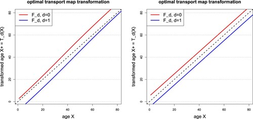
Table 3 presents the prediction accuracy of the OT input transformed models. At first sight it is surprising that the input OT transformed model $\hat{\mu }({\mathit{X}}_{+})$ has a better predictive performance than the unawareness price model $\mu (\mathit{X})$. However, by considering the details of the true model, this is not that surprising. Women have generally higher costs than men at the same age $\mathit{X}=X$ under model assumption (15(15) $Y{|}_{(\mathit{X},\mathit{D})}\sim \mathcal{N}(X+20(1-D){\mathbb{1}}_{X\in [20,40]}-10D,100).$(15) ), and considering the age shifts of the OT maps makes women and men more similar with respect to claim costs in this example. The MSE of the unawareness price $\mu (\mathit{X})$ is calculated as $\begin{array}{rl}\mathbb{E}\left[{(Y-\mu (\mathit{X}))}^2\right]& =\mathbb{E}\left[\mathbb{E}[{(Y-\mu (\mathit{X},\mathit{D})+\mu (\mathit{X},\mathit{D})-\mu (\mathit{X}))}^2|\mathit{X},\mathit{D}]\right]\\ & =\mathbb{E}\left[{(Y-\mu (\mathit{X},\mathit{D}))}^2\right]+\mathbb{E}\left[{(\mu (\mathit{X},\mathit{D})-\mu (\mathit{X}))}^2\right].\end{array}$The first term on the right hand side is the MSE of the best-estimate predictor $\mu (\mathit{X},\mathit{D})$ based on all information $(\mathit{X},\mathit{D})$, and the second term corresponds to the loss of accuracy by using the unawareness price $\mu (\mathit{X})$. The OT maps (31(31) $F_{+}(x)=\frac{1}{2}\mathrm{\Phi }\left(\frac{x-x_0}{\tau }\right)+\frac{1}{2}\mathrm{\Phi }\left(\frac{x-x_1}{\tau }\right),$(31) ) and (32(32) $F_{+}(x)=\frac{1}{2}\mathrm{\Phi }\left(\frac{x-(x_0+x_1)/2}{\tau }\right).$(32) ) make women older and men younger, and as a result their risk profiles with respect to the transformed inputs ${\mathit{X}}_{+}=T_{\mathit{d}}(\mathit{X})$ become more similar in this example. This precisely leads, in this case, to a smaller MSE of $\hat{\mu }({\mathit{X}}_{+})$ over $\mu (\mathit{X})$. Namely, we have (33) $\mathbb{E}\left[{(Y-\hat{\mu }({\mathit{X}}_{+}))}^2\right]=\mathbb{E}\left[{(Y-\mu (\mathit{X},\mathit{D}))}^2\right]+\mathbb{E}\left[{(\mu (\mathit{X},\mathit{D})-\hat{\mu }({\mathit{X}}_{+}))}^2\right],$(33) with the last term being smaller than the last one in the unawareness price case because the $\mathit{d}$-dependent transformation ${\mathit{X}}_{+}=T_{\mathit{d}}(\mathit{X})$ makes $\hat{\mu }({\mathit{X}}_{+})$ more similar to $\mu (\mathit{X},\mathit{D})$ compared to $\mu (\mathit{X})$. This is specific to our example which can be better understood by discussing Figure 6. Figure 6 illustrates the OT input transformed model prices $\hat{\mu }({\mathit{X}}_{+})$ for choices (31(31) $F_{+}(x)=\frac{1}{2}\mathrm{\Phi }\left(\frac{x-x_0}{\tau }\right)+\frac{1}{2}\mathrm{\Phi }\left(\frac{x-x_1}{\tau }\right),$(31) )–(32(32) $F_{+}(x)=\frac{1}{2}\mathrm{\Phi }\left(\frac{x-(x_0+x_1)/2}{\tau }\right).$(32) ) for $F_{+}$. For Figure 6 we map these prices back to the original features $\mathit{X}$, separated by gender $\mathit{D}$. This back-transformation can be done because the OT maps $T_{\mathit{d}}$ are one-to-one under continuous non-protected covariates $\mathit{X}$, and for given $\mathit{D}=\mathit{d}$, see Remarks 3.1. Figure 6 then evaluates the prices $\hat{\mu }({\mathit{X}}_{+})$, where we consider ${\mathit{X}}_{+}={\mathit{X}}_{+}(\mathit{x};\mathit{d})=T_{\mathit{d}}(\mathit{x})$ as a function of age $\mathit{x}$ for fixed gender $\mathit{D}=\mathit{d}$. The right hand side shows choice (32(32) $F_{+}(x)=\frac{1}{2}\mathrm{\Phi }\left(\frac{x-(x_0+x_1)/2}{\tau }\right).$(32) ) for $F_{+}$, which leads to parallel shifts for the transformed age assignments ${\mathit{X}}_{+}$, see Figure 5 (rhs). As a consequence, the excess pregnancy costs of women with ages in $[20,40]$ are shared with men having ages in $[30,50]$ in our example, see orange and cyan lines in Figure 6 (rhs). This should be contrasted to the DFIP ${\mu }^{\ast }(\mathit{X})$ (green line in Figure 2) which shares the excess pregnancy costs within the age class $[20,40]$ for both genders. The transformation for choice (31(31) $F_{+}(x)=\frac{1}{2}\mathrm{\Phi }\left(\frac{x-x_0}{\tau }\right)+\frac{1}{2}\mathrm{\Phi }\left(\frac{x-x_1}{\tau }\right),$(31) ) for $F_{+}$ leads to a distortion along the age cohorts as we do not have parallel shifts, see Figures 5 (lhs) and 6 (lhs).

Coming back to (33(33) $\mathbb{E}\left[{(Y-\hat{\mu }({\mathit{X}}_{+}))}^2\right]=\mathbb{E}\left[{(Y-\mu (\mathit{X},\mathit{D}))}^2\right]+\mathbb{E}\left[{(\mu (\mathit{X},\mathit{D})-\hat{\mu }({\mathit{X}}_{+}))}^2\right],$(33) ) and focusing on choice (32(32) $F_{+}(x)=\frac{1}{2}\mathrm{\Phi }\left(\frac{x-(x_0+x_1)/2}{\tau }\right).$(32) ) for $F_{+}$, which corresponds to Figure 5 (rhs), we observe that the age shifts of 5 years lead to OT input transformed prices $\hat{\mu }({\mathit{X}}_{+})$ that rather perfectly match the best-estimates $\mu (\mathit{X},\mathit{D})$. In fact, the age shifts of 5 years exactly compensate the term $-10D$ in (15(15) $Y{|}_{(\mathit{X},\mathit{D})}\sim \mathcal{N}(X+20(1-D){\mathbb{1}}_{X\in [20,40]}-10D,100).$(15) ), and the only difference between women and men (after the age shifts) are the pregancy related costs. This explains the good MSE results of input OT in Table 3, but this is very model specific here, as can be verified by switching the age profiles (i.e. by setting $x_0=45$ and $x_1=35$) and keeping everything else unchanged.

Figure 6. OT input transformed model prices $\hat{\mu }({\mathit{X}}_{+})$ for examples (31(31) $F_{+}(x)=\frac{1}{2}\mathrm{\Phi }\left(\frac{x-x_0}{\tau }\right)+\frac{1}{2}\mathrm{\Phi }\left(\frac{x-x_1}{\tau }\right),$(31) )–(32(32) $F_{+}(x)=\frac{1}{2}\mathrm{\Phi }\left(\frac{x-(x_0+x_1)/2}{\tau }\right).$(32) ) of $F_{+}$.

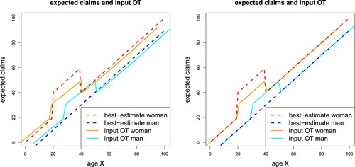
Table 3. MSEs and average prediction of the different prices in Example 2.14.

Average price	MSE	Average price
Best-estimate price $\mu (\mathit{X},\mathit{D})$	100.00	41.25
Unawareness price $\mu (\mathit{X})$	197.20	41.25
Input OT map of (31(31) $F_{+}(x)=\frac{1}{2}\mathrm{\Phi }\left(\frac{x-x_0}{\tau }\right)+\frac{1}{2}\mathrm{\Phi }\left(\frac{x-x_1}{\tau }\right),$(31) ) for $\hat{\mu }({\mathit{X}}_{+})$	162.77	41.25
Input OT map of (32(32) $F_{+}(x)=\frac{1}{2}\mathrm{\Phi }\left(\frac{x-(x_0+x_1)/2}{\tau }\right).$(32) ) for $\hat{\mu }({\mathit{X}}_{+})$	162.72	41.25
Input OT map of (32(32) $F_{+}(x)=\frac{1}{2}\mathrm{\Phi }\left(\frac{x-(x_0+x_1)/2}{\tau }\right).$(32) ) for best-estimate $\hat{\mu }({\mathit{X}}_{+},\mathit{D})$	100.60	41.24

Figure 7 shows the results of the switched age profile case, with women having a higher average age, $x_0=45$, than men, $x_1=35$. This leads to the opposite behaviour for the conditional probabilities $\mathbb{P}(D=0|X=x)$, see Figure 7 (lhs), and, equivalently, for the unawareness price, see Figure 7 (middle). On the other hand, the DFIP is not affected by this change as we do not infer D from X (we do not proxy discriminate in the DFIP). Figure 7 (rhs) shows the resulting OT input transformed prices $\hat{\mu }({\mathit{X}}_{+})$ for example (32(32) $F_{+}(x)=\frac{1}{2}\mathrm{\Phi }\left(\frac{x-(x_0+x_1)/2}{\tau }\right).$(32) ) of $F_{+}$. These OT input transformed prices now provide a worse MSE (33(33) $\mathbb{E}\left[{(Y-\hat{\mu }({\mathit{X}}_{+}))}^2\right]=\mathbb{E}\left[{(Y-\mu (\mathit{X},\mathit{D}))}^2\right]+\mathbb{E}\left[{(\mu (\mathit{X},\mathit{D})-\hat{\mu }({\mathit{X}}_{+}))}^2\right],$(33) ) compared to the unawareness price, see also Table 4. This also verified by Figure 7. Figure 7 and Table 4 may not be in support of using OT input transformation generally, however, we emphasize that the OT map $T_{\mathit{d}}$ is selected solely based on the inputs $(\mathit{X},\mathit{D})$ and not considering the response Y. As a result, we can receive a predictive model that is either better or worse than the unawareness price model. This is, however, not surprising, since input OT targets demographic parity, not predictive performance. In fact, the selection of the OT map is not even allowed to consider the response Y, otherwise it may (and will) imply a sort of indirect model selection discrimination.

The prices depicted in Figures 6 and 7 (rhs) satisfy demographic parity and avoid proxy discrimination with respect to $({\mathit{X}}_{+},\mathit{D})$, see Proposition 3.2. As discussed in Remarks 3.1, whether one considers these prices desirable in relation to direct and proxy discrimination depends on whether the transformed age ${\mathit{X}}_{+}$ can be interpreted/justified as a valid covariate in its own right. If it is seen as just an artefact of the dependence structure of $(\mathit{X},\mathit{D})$, stakeholders may be more interested in discrimination with respect to the original covariates $(\mathit{X},\mathit{D})$. From such a perspective it is clear that the prices of Figures 6 and 7 (rhs) are subject to even direct discrimination, given the different dashed lines for women and for men on the original scale.

Figure 7. Changed age profiles with $x_0=45$ (women) and $x_1=35$ (men): (lhs) conditional probability $\mathbb{P}(D=0|X=x)$ as a function of $x\in \mathbb{R}$; (middle) best-estimate, unawareness and discrimination-free insurance prices; (rhs) OT input transformed model prices $\hat{\mu }({\mathit{X}}_{+})$ for example (32(32) $F_{+}(x)=\frac{1}{2}\mathrm{\Phi }\left(\frac{x-(x_0+x_1)/2}{\tau }\right).$(32) ) of $F_{+}$.

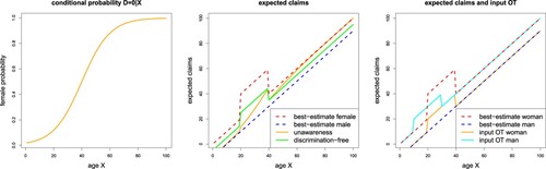
Table 4. Changed role of ages of women and men, setting $x_0=45$ and $x_1=35$.

price Π	MSE	average price
Best-estimate price $\mu (\mathit{X},\mathit{D})$	100.00	38.01
Unawareness price $\mu (\mathit{X})$	197.12	38.01
Input OT map of (31(31) $F_{+}(x)=\frac{1}{2}\mathrm{\Phi }\left(\frac{x-x_0}{\tau }\right)+\frac{1}{2}\mathrm{\Phi }\left(\frac{x-x_1}{\tau }\right),$(31) ) for $\hat{\mu }({\mathit{X}}_{+})$	290.68	38.01
Input OT map of (32(32) $F_{+}(x)=\frac{1}{2}\mathrm{\Phi }\left(\frac{x-(x_0+x_1)/2}{\tau }\right).$(32) ) for $\hat{\mu }({\mathit{X}}_{+})$	290.64	38.01

An important difference between the DFIP ${\mu }^{\ast }(\mathit{X})$ and the OT map transformed prices $\hat{\mu }({\mathit{X}}_{+})$ is that the latter always provide a (statistically) unbiased model, if the chosen regression class is sufficiently flexible. In fact, $\hat{\mu }({\mathit{X}}_{+})$ may not only satisfy the balance property, but even the more restrictive auto-calibration property; see (Wüthrich & Ziegel, 2024).

Finally, we build a best-estimate model $\hat{\mu }({\mathit{X}}_{+},\mathit{D})$ on the transformed information $({\mathit{X}}_{+},\mathit{D})$. We do this by separately fitting two cubic splines to the women data $(Y,X_{+},D=0)$ and the men data $(Y,X_{+},D=1)$, respectively. The results are presented on the last line of Table 3. Up to estimation error, we rediscover the true model, but on the transformed input data, as the MSE only contains the noise part (irreducible risk) of the response Y. Thus, as expected, this one-to-one OT map (in the continuous case), for given gender, does not involve a loss of information, and the predictive performance in the parametrizations $(\mathit{X},\mathit{D})$ and $({\mathit{X}}_{+},\mathit{D})$ coincides (up to estimation error).

Remark 3.4

For OT input tranformation we need to select an unconditional distribution $F_{+}$, see (25(25) ${{\mathit{X}}_{+}|}_{\mathit{D}}\sim F_{+}\left(\mathit{x}\right),$(25) ). In Example 3.3 we have provided two natural choices (31(31) $F_{+}(x)=\frac{1}{2}\mathrm{\Phi }\left(\frac{x-x_0}{\tau }\right)+\frac{1}{2}\mathrm{\Phi }\left(\frac{x-x_1}{\tau }\right),$(31) )–(32(32) $F_{+}(x)=\frac{1}{2}\mathrm{\Phi }\left(\frac{x-(x_0+x_1)/2}{\tau }\right).$(32) ), but we have not discussed a systematic way of choosing this unconditional distribution $F_{+}$. Intuitively, the OT transformed covariates ${\mathit{X}}_{+}$ should be as close as possible to $\mathit{X}$, and at the same time they should be independent from $\mathit{D}$ under $\mathbb{P}$, i.e. ${\mathit{X}}_{+}\perp \perp \mathit{D}$. This is a problem studied in Delbaen and Majumdar (2023): (34) $\underset{\mathit{Z}\perp \perp \mathit{D}}{\arg min}{\Vert \mathit{X}-\mathit{Z}\Vert }_2,$(34) for the $L^2$-distance function $\Vert \cdot {\Vert }_2$ under $\mathbb{P}$. Theorems 5–7 of Delbaen and Majumdar (2023) show that such a minimum can be found by solving a related problem involving the Wasserstein distance (26(26) ${\mathcal{W}}_2(F_{\mathit{d}},F_{+}):={(\underset{{\pi }_{\mathit{d}}\in {\mathcal{P}}_{\mathit{d}}}{inf}\int \varrho (\mathit{x},{\mathit{x}}_{+}{)}^2\mathrm{d}{\pi }_{\mathit{d}}(\mathit{x},{\mathit{x}}_{+}))}^{1/2},$(26) ) with the Euclidean distance for ϱ. Unfortunately, this is still only a mathematical result and no efficient algorithm is currently known to calculate this solution in higher dimensions.

From an actuarial viewpoint, it is not fully clear whether (34(34) $\underset{\mathit{Z}\perp \perp \mathit{D}}{\arg min}{\Vert \mathit{X}-\mathit{Z}\Vert }_2,$(34) ) solves the right problem, as this may depend on the chosen class of regression functions. e.g. if we work with GLMs then certain real-valued covariates may be considered on the original scale and others on the log-scale, which may/should impact the choice of the objective function in (34(34) $\underset{\mathit{Z}\perp \perp \mathit{D}}{\arg min}{\Vert \mathit{X}-\mathit{Z}\Vert }_2,$(34) ). Moreover, categorical covariates may pose further challenges in defining suitable objective functions. Concluding, the problem of selecting the OT input transformation in a systematic way is still an open problem that requires more research which goes beyond the scope of this article.

3.3. Model post-processing

Model post-processing to achieve fairness works on the outputs, and not on the inputs like data pre-processing. From a purely technical viewpoint, both methods work in a similar manner. A main difference is that input pre-processing usually is multi-dimensional and (regression) model post-processing is one-dimensional. Assume, in a first step, we have fitted a best-estimate price model $(\mathit{X},\mathit{D})\mapsto \mu (\mathit{X},\mathit{D})$. Model post-processing applies transformations to these best-estimate prices $\mu (\mathit{X},\mathit{D})\mapsto {\mu }_{+}$ such that the transformed price ${\mu }_{+}$ fulfils a fairness axiom. Focusing on demographic parity, the transformed price ${\mu }_{+}$ should be independent of $\mathit{D}$ under $\mathbb{P}$. Note that any of the following steps could equivalently be applied to any other pricing functional, such as the unawareness price $\mu (\mathit{X})$.

If we apply an OT output transformation, we modify (24(24) ${\mathit{X}}_{\mathit{d}}:={\mathit{X}|}_{\{\mathit{D}=\mathit{d}\}}\sim F_{\mathit{d}}(\mathit{x}):=F(\mathit{x}|\mathit{D}=\mathit{d}),$(24) ) and (25(25) ${{\mathit{X}}_{+}|}_{\mathit{D}}\sim F_{+}\left(\mathit{x}\right),$(25) ) as follows. For $\mathit{d}\in \mathfrak{D}$, we change the conditional distributions $G_{\mathit{d}}$ on $\mathbb{R}$ (35) ${\mu }_{\mathit{d}}(\mathit{X}):={\mu (\mathit{X},\mathit{D})|}_{\{\mathit{D}=\mathit{d}\}}\sim G_{\mathit{d}}(m):=\mathbb{P}(\mu (\mathit{X},\mathit{D})\le m|\mathit{D}=\mathit{d})\mathrm{for}m\in \mathbb{R},$(35) to an unconditional distribution $G_{+}$ for the prices (36) ${{\mu }_{+}|}_{\mathit{D}}\sim G_{+}\left(m\right).$(36) In particular, this means that the real-valued random variable ${\mu }_{+}\sim G_{+}$ is independent of $\mathit{D}$. Based on these choices we look for OT maps $T_{\mathit{d}}:{\mu }_{\mathit{d}}(\mathit{X})\mapsto {\mu }_{+}$, given $\mathit{d}\in \mathfrak{D}$, providing the corresponding distribution. Since everything is one-dimensional here, we can directly work with versions (28(28) $X\mapsto X_{+}=T_{\mathit{d}}(X)=F_{+}^{-1}\circ F_{\mathit{d}}(X).$(28) ) and (29(29) $V:=F_{\mathit{d}}(X_{-})+U(F_{\mathit{d}}(X_{-})-F_{\mathit{d}}(X)),$(29) ), respectively, depending on whether our price functionals ${\mu }_{\mathit{d}}(\mathit{X})$ have continuous marginals $G_{\mathit{d}}$ or not. Thus, in the continuous case we have OT maps (37) ${\mu }_{\mathit{d}}(\mathit{X})\mapsto {\mu }_{+}=T_{\mathit{d}}({\mu }_{\mathit{d}}(\mathit{X}))=G_{+}^{-1}\circ G_{\mathit{d}}({\mu }_{\mathit{d}}(\mathit{X})),$(37) for $\mathit{d}\in \mathfrak{D}$. The resulting Wasserstein distance is given by (27(27) $\begin{array}{rl}{\mathcal{W}}_2(F_{\mathit{d}},F_{+})& ={\left({\int }_0^1{(F_{\mathit{d}}^{-1}(q)-F_{+}^{-1}(q))}^2\mathrm{d}q\right)}^{1/2}\\ & =\mathbb{E}{\left[{(F_{\mathit{d}}^{-1}(U)-F_{+}^{-1}(U))}^2\right]}^{1/2},\end{array}$(27) ) with $(F_{\mathit{d}},F_{+})$ replaced by $(G_{\mathit{d}},G_{+})$. With this procedure, since the distribution $G_{+}$ does not depend on $\mathit{D}$, the OT transformed price ${\mu }_{+}$ fulfills demographic parity. The remaining question is how to choose $G_{+}$, this is discussed below.

Remark 3.5

${\mu }_{\mathit{d}}(\mathit{X})\sim G_{\mathit{d}}$ is a real-valued random variable, and one should not get confused by the multi-dimensional covariate $\mathit{X}$ in this expression; also the OT transformed price ${\mu }_{+}\sim G_{+}$ is a real-valued random variable, independent of $\mathit{D}$. Often, one wants to relate this price ${\mu }_{+}$ to the original covariates $(\mathit{X},\mathit{D})$. In the continuous case we can do this using the OT maps (37(37) ${\mu }_{\mathit{d}}(\mathit{X})\mapsto {\mu }_{+}=T_{\mathit{d}}({\mu }_{\mathit{d}}(\mathit{X}))=G_{+}^{-1}\circ G_{\mathit{d}}({\mu }_{\mathit{d}}(\mathit{X})),$(37) ), namely, we have a measurable map (38) $(\mathit{x},\mathit{d})\mapsto {\mu }_{+}={\mu }_{+}(\mathit{x};\mathit{d})=G_{+}^{-1}\circ G_{\mathit{d}}(\mu (\mathit{x},\mathit{d}))\in \mathbb{R}.$(38) Formula (38(38) $(\mathit{x},\mathit{d})\mapsto {\mu }_{+}={\mu }_{+}(\mathit{x};\mathit{d})=G_{+}^{-1}\circ G_{\mathit{d}}(\mu (\mathit{x},\mathit{d}))\in \mathbb{R}.$(38) ) gives the OT transformed price ${\mu }_{+}$ of a given insurance policy with covariates $(\mathit{X},\mathit{D})=(\mathit{x},\mathit{d})$, and (37(37) ${\mu }_{\mathit{d}}(\mathit{X})\mapsto {\mu }_{+}=T_{\mathit{d}}({\mu }_{\mathit{d}}(\mathit{X}))=G_{+}^{-1}\circ G_{\mathit{d}}({\mu }_{\mathit{d}}(\mathit{X})),$(37) ) describes the distribution of this price, if we randomly select an insurance policy from our portfolio $\mathit{X}{|}_{\{\mathit{D}=\mathit{d}\}}\sim F_{\mathit{d}}$, for given protected attributes $\mathit{D}=\mathit{d}$.

Example 3.6

Application of output OT

We revisit Examples 2.14 and 3.3, but now, instead of input pre-processing, we apply model post-processing to the best-estimate $\mu (\mathit{X},\mathit{D})$. These best-estimates are illustrated in red and blue colour in Figure 2. As density $g_{+}$ we simply choose the average of the two conditional densities (39) $g_{+}(m)=\frac{1}{2}(g_0(m)+g_1(m))\mathrm{for}m\in \mathbb{R}.$(39) Note that the distributions of $\mu (X,D){|}_{\{D=d\}}$ are absolutely continuous, therefore their densities $g_d$ exist. Figure 8 illustrates the density $g_{+}$ and the resulting distribution $G_{+}$, respectively.

Figure 8. OT output post-processing density $g_{+}$ and distribution $G_{+}$.

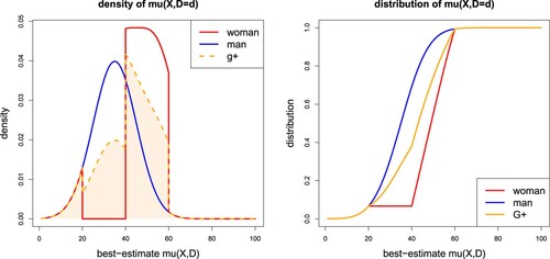
Table 5 presents the results of the OT output post-processed best-estimate prices using density (39(39) $g_{+}(m)=\frac{1}{2}(g_0(m)+g_1(m))\mathrm{for}m\in \mathbb{R}.$(39) ) for $g_{+}$. The resulting MSE is smaller than the corresponding value of the input OT version, see Table 3. This is generally expected for suitable choices of $g_{+}$ because the fairness debiasing only takes place in the last step of the (estimation) procedure, and all previous steps deriving the best-estimate price uses full information $(\mathit{X},\mathit{D})$. Input OT already performs the debiasing procedure in the first step and, therefore, all subsequent steps are generally non-optimal in terms of full information $(\mathit{X},\mathit{D})$. OT output post-processing directly acts on the best-estimate prices $\mu (\mathit{X},\mathit{D})$. These best-estimate prices can be understood as price cohorts, and for OT output post-processing the specific (multi-dimensional) value of the non-protected covariates, say $\mathit{X}\in \{\mathit{x},{\mathit{x}}^{\prime }\}$, does not matter as long as they belong to the same price cohort $\mu (\mathit{X}=\mathit{x},\mathit{D}=\mathit{d})=\mu (\mathit{X}={\mathit{x}}^{\prime },\mathit{D}=\mathit{d})$. In case of non-monotone best-estimate prices, this can lead to price distortions that are not easily explainable to customers and policymakers. In Figure 9 (top) we express the output post-processed prices ${\mu }_{+}={\mu }_{+}(\mathit{x};\mathit{d})$ as a function of the original age variable $\mathit{X}=\mathit{x}$, separated by gender $\mathit{D}=\mathit{d}\in \{0,1\}$, we also refer to (38(38) $(\mathit{x},\mathit{d})\mapsto {\mu }_{+}={\mu }_{+}(\mathit{x};\mathit{d})=G_{+}^{-1}\circ G_{\mathit{d}}(\mu (\mathit{x},\mathit{d}))\in \mathbb{R}.$(38) ). We observe that for women $\mathit{D}=0$, the best-estimate prices $\mu (\mathit{X}=30,\mathit{D}=0)=\mu (\mathit{X}=50,\mathit{D}=0)=50$ coincide (red dots in Figure 9, top), but the underlying risk factors for these high costs are completely different ones. Women at age 30 have high costs because of pregnancy, and women at age 50 have high costs because of aging (women at age 50 are assumed to not be able to get pregnant). Using OT output post-processing, these two age classes (being in the same price cohort) are treated completely equally and obtain the same fairness debiasing discount (orange dot in Figure 9, top). But this discount for women at age 50 cannot be justified if we believe that fairness (or anti-discrimination) should compensate for the excess pregnancy costs which only applies to women but not to men between ages 20 and 40. In fact, this is precisely how the excess pregnancy costs are treated in the DFIP ${\mu }^{\ast }(\mathit{X})$, see green line in Figure 9 (bottom-rhs), and in the OT input pre-processing price $\mu ({\mathit{X}}_{+})$, see Figure 9 (bottom-lhs); the plots at the bottom of Figure 9 are repeated from Examples 2.14 and 3.3 for ease of comparison.

Remark 3.7

From Example 3.6, we conclude that output post-processing should be used with great care. The price functional $\mathit{x}\mapsto \mu (\mathit{X}=\mathit{x},\mathit{d})\in \mathbb{R}$ typically leads to a large loss of information (this can be interpreted as a projection), and insurance policies with completely different risk factors may be assigned to the same price cohort by this projection. Therefore, it is questionable if model post-processing should treat different covariate cohorts $\mathit{X}=\mathit{x}$ with equal best-estimate prices equally (which precisely happens in OT output post-processing) or whether we should look for another way of correcting. Of course, one may similarly object to the case of input OT, particularly that excess pregnancy costs of women at age 20-40 are shared specifically with men of age 30–50. Nonetheless, at least, the results of input OT, Figure 9 (bottom-lhs), are easier to interpret compared to Figure 9 (top). Note though that when policyholder features $\mathit{X}$ are highly granular, it becomes difficult to assign policies into homogeneous groups. In such circumstances we may find that the new rating classes induced by input OT are also hard to interpret.

Figure 9. (Top) OT output post-processed prices ${\mu }_{+}={\mu }_{+}(\mathit{x};\mathit{d})$ expressed in their original features $\mathit{x}$ and separated by gender $\mathit{d}$, see (38(38) $(\mathit{x},\mathit{d})\mapsto {\mu }_{+}={\mu }_{+}(\mathit{x};\mathit{d})=G_{+}^{-1}\circ G_{\mathit{d}}(\mu (\mathit{x},\mathit{d}))\in \mathbb{R}.$(38) ); (bottom-lhs) OT input pre-processing taken from Figure 6; (bottom-rhs) unawareness price and DFIP taken from Figure 2.

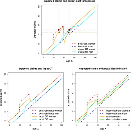
Table 5. MSEs and average prediction of the different prices in Example 2.14.

price Π	MSE	average price
Best-estimate price $\mu (\mathit{X},\mathit{D})$	100.00	41.25
Unawareness price $\mu (\mathit{X})$	197.20	41.25
Output OT map of (39(39) $g_{+}(m)=\frac{1}{2}(g_0(m)+g_1(m))\mathrm{for}m\in \mathbb{R}.$(39) ) for ${\mu }_{+}$	152.97	41.25

If, despite the last criticism, we would like to hold on to OT model post-processing, we may ask the question about the optimal OT transform in (37(37) ${\mu }_{\mathit{d}}(\mathit{X})\mapsto {\mu }_{+}=T_{\mathit{d}}({\mu }_{\mathit{d}}(\mathit{X}))=G_{+}^{-1}\circ G_{\mathit{d}}({\mu }_{\mathit{d}}(\mathit{X})),$(37) ) and (36(36) ${{\mu }_{+}|}_{\mathit{D}}\sim G_{+}\left(m\right).$(36) ), respectively, to receive maximal predictive power of $\hat{\mu }$ for Y. This is the same question as discussed in Remark 3.4 for OT input pre-processing. The question of optimal maps for input OT pre-processing could not be generally answered because of potential high-dimensionality, non-linearity and computational complexity, see Remark 3.4. However, for optimal (one-dimensional) model post-processing with OT we can rely on (simpler) analytical results in one-dimensional OT. In particular, Theorem 2.3 of Chzhen et al. (2020) states the following.

Proposition 3.8

Assume ${\mu }_{\mathit{d}}(\mathit{X})\sim G_{\mathit{d}}$ are absolutely continuous for all $\mathit{d}\in \mathfrak{D}$. Consider (40) ${\mu }_{+}(\mathit{x};\mathit{d})=\left(\sum _{{\mathit{d}}^{\prime }\in \mathfrak{D}}\mathbb{P}(\mathit{D}={\mathit{d}}^{\prime })G_{{\mathit{d}}^{\prime }}^{-1}\right)\circ G_{\mathit{d}}(\mu (\mathit{x},\mathit{d})).$(40) Then, ${\mu }_{+}={\mu }_{+}(\mathit{X},\mathit{D})$ is the $\sigma (\mathit{X},\mathit{D})$-measurable and demographic parity fair predictor of Y that has minimal MSE.

Remarks 3.9

• The big round brackets in (40(40) ${\mu }_{+}(\mathit{x};\mathit{d})=\left(\sum _{{\mathit{d}}^{\prime }\in \mathfrak{D}}\mathbb{P}(\mathit{D}={\mathit{d}}^{\prime })G_{{\mathit{d}}^{\prime }}^{-1}\right)\circ G_{\mathit{d}}(\mu (\mathit{x},\mathit{d})).$(40) ) give the inverse of the optimal distribution for $G_{+}$, see also (37(37) ${\mu }_{\mathit{d}}(\mathit{X})\mapsto {\mu }_{+}=T_{\mathit{d}}({\mu }_{\mathit{d}}(\mathit{X}))=G_{+}^{-1}\circ G_{\mathit{d}}({\mu }_{\mathit{d}}(\mathit{X})),$(37) ). In fact, this specific choice of $G_{+}$ corresponds to the barycenter of the conditional distributions $(G_{\mathit{d}}{)}_{\mathit{d}\in \mathfrak{D}}$ with respect to the Wasserstein distance (27(27) $\begin{array}{rl}{\mathcal{W}}_2(F_{\mathit{d}},F_{+})& ={\left({\int }_0^1{(F_{\mathit{d}}^{-1}(q)-F_{+}^{-1}(q))}^2\mathrm{d}q\right)}^{1/2}\\ & =\mathbb{E}{\left[{(F_{\mathit{d}}^{-1}(U)-F_{+}^{-1}(U))}^2\right]}^{1/2},\end{array}$(27) ). From this we conclude that if we choose this barycenter, we receive the $L^2$-optimal $\mathit{D}$-independent $\sigma (\mathit{X},\mathit{D})$-measurable predictor for Y, satisfying demographic parity. Since choice (39(39) $g_{+}(m)=\frac{1}{2}(g_0(m)+g_1(m))\mathrm{for}m\in \mathbb{R}.$(39) ) is not the barycenter in that example, predictive performance could still be improved in our OT model post-processing example. On the other hand, we have used the barycenter in (32(32) $F_{+}(x)=\frac{1}{2}\mathrm{\Phi }\left(\frac{x-(x_0+x_1)/2}{\tau }\right).$(32) ), see also Table 2, but for input pre-processing this is not a crucial choice and other choices may perform better (depending on the specific regression model class being used).

• In (40(40) ${\mu }_{+}(\mathit{x};\mathit{d})=\left(\sum _{{\mathit{d}}^{\prime }\in \mathfrak{D}}\mathbb{P}(\mathit{D}={\mathit{d}}^{\prime })G_{{\mathit{d}}^{\prime }}^{-1}\right)\circ G_{\mathit{d}}(\mu (\mathit{x},\mathit{d})).$(40) ) we have a measurable function of type (38(38) $(\mathit{x},\mathit{d})\mapsto {\mu }_{+}={\mu }_{+}(\mathit{x};\mathit{d})=G_{+}^{-1}\circ G_{\mathit{d}}(\mu (\mathit{x},\mathit{d}))\in \mathbb{R}.$(38) ). We can relate this back to conditional expectations similar to Proposition 3.2. Consider the random variable ${\mu }^{†}(\mathit{X};{\mathit{d}}^{\prime }):=G_{{\mathit{d}}^{\prime }}^{-1}\circ G_{\mathit{d}}({\mu }_{\mathit{d}}(\mathit{X}))\sim G_{{\mathit{d}}^{\prime }},$i.e. this random variable ${\mu }^{†}(\mathit{X};{\mathit{d}}^{\prime })$ has the same conditional distribution as ${\mu }_{{\mathit{d}}^{\prime }}(\mathit{X})$. We can then rewrite (40(40) ${\mu }_{+}(\mathit{x};\mathit{d})=\left(\sum _{{\mathit{d}}^{\prime }\in \mathfrak{D}}\mathbb{P}(\mathit{D}={\mathit{d}}^{\prime })G_{{\mathit{d}}^{\prime }}^{-1}\right)\circ G_{\mathit{d}}(\mu (\mathit{x},\mathit{d})).$(40) ) as follows ${\mu }_{+}(\mathit{X};\mathit{d})=\left(\sum _{{\mathit{d}}^{\prime }\in \mathfrak{D}}\mathbb{P}(\mathit{D}={\mathit{d}}^{\prime })G_{{\mathit{d}}^{\prime }}^{-1}\right)\circ G_{\mathit{d}}({\mu }_{\mathit{d}}(\mathit{X}))=\sum _{{\mathit{d}}^{\prime }\in \mathfrak{D}}{\mu }^{†}(\mathit{X};{\mathit{d}}^{\prime })\mathbb{P}(\mathit{D}={\mathit{d}}^{\prime }).$That is, similar to the DFIP and the OT input pre-processed price of Proposition 3.2, we take an unconditional expectation in protected attributes $\mathit{D}$ over ${\mu }^{†}(\mathit{X};{\mathit{d}}^{\prime })$. Moreover, we can relate the latter to best-estimate prices, i.e. to any realization of ${\mathit{X}}_{\mathit{d}}=\mathit{x}$ we can assign a covariate value ${\mathit{x}}_{{\mathit{d}}^{\prime }}^{†}$ such that ${\mu }^{†}(\mathit{x};{\mathit{d}}^{\prime })=\mathbb{E}\left[Y|\mathit{X}={\mathit{x}}_{{\mathit{d}}^{\prime }}^{†},\mathit{D}={\mathit{d}}^{\prime }\right]=\mu ({\mathit{x}}_{{\mathit{d}}^{\prime }}^{†},{\mathit{d}}^{\prime }).$This implies, ${\mu }_{+}(\mathit{x};\mathit{d})=\sum _{{\mathit{d}}^{\prime }\in \mathfrak{D}}\mu ({\mathit{x}}_{{\mathit{d}}^{\prime }}^{†},{\mathit{d}}^{\prime })\mathbb{P}(\mathit{D}={\mathit{d}}^{\prime }).$Thus, formally we can write the OT post-processed price as a DFIP. However, this line of argument suffers the same deficiency as Figure 9 (top), namely, the assignment ${\mathit{x}}_{{\mathit{d}}^{\prime }}^{†}$ is non-unique, and we may select different non-protected covariate values for this assignment that have completely different risk factors.

4. Conclusions and discussion

We have shown that direct and proxy discrimination and group fairness are materially different concepts. We can have discrimination-free insurance prices that do not satisfy any of the group fairness axioms, and, vice versa, we can have, e.g. prices that satisfy demographic parity but are subject to material proxy discrimination and even direct discrimination. In particular, in Example 2.21 we gave an example of a price that satisfies demographic parity, equalized odds and predictive parity, but directly discriminates from an insurance regulation view. This clearly questions the direct application of group fairness axioms to insurance pricing, as they do not provide a quick fix for (and may even conflict with) mitigating direct and proxy discrimination.

In a next step, we presented OT input pre-processing and OT output post-processing. These methods can be used to make distributions of non-protected characteristics independent of protected attributes. Input pre-processing locally perturbs the non-protected covariates $\mathit{X}{|}_{\mathit{D}}$ such that the resulting conditional distributions become independent of the protected attributes $\mathit{D}$. If we only work with these transformed covariates, we receive prices that satisfy demographic parity and avoid proxy discrimination; however note that there will generally be direct discrimination with respect to the original covariates, as depicted in Figure 9. Output post-processing is different as it acts on the real-valued best-estimates $\mu (\mathit{X},\mathit{D})$, which should be seen as a summary statistic for pricing that already suffers from a loss of information, i.e. we can no longer fully distinguish the underlying risk factors that lead to these best-estimate prices. This may make output post-processing problematic because we may receive a fairness debiasing that cannot be explained to customers and policymakers.

The following table compares the crucial differences between discrimination-free insurance pricing and group fairness through OT input pre-processing.

Table

Addressing proxy discrimination	Addressing fairness
Model post-processing of prices $\mu (\mathit{X},\mathit{D})$	Input pre-processing of features $\mathit{X}$
Change of probability from $\mathbb{P}$ to ${\mathbb{P}}^{\ast }$	Deformation of $\mathit{X}$ to ${\mathit{X}}_{+}$
Independence of $\mathit{X}$ and $\mathit{D}$ under ${\mathbb{P}}^{\ast }$	Independence of ${\mathit{X}}_{+}$ and $\mathit{D}$ under $\mathbb{P}$
Dependence of $\mathit{X}$ and $\mathit{D}$ under $\mathbb{P}$ ···	Dependence of $\mathit{X}$ and $\mathit{D}$ under $\mathbb{P}$ ···
···  does not matter for price adjustments	···  matters for price adjustments

We list further points that require a careful consideration in any attempt to regulate insurance prices with reference to non-discrimination and group fairness concepts:

• One difficulty in this field is that there are many different terms that do not have precise (mathematical) definitions or, even worse, their definitions contradict. Therefore, it would be beneficial to have a unified framework and consistent definitions, e.g. for terms such as disparate effect, disparate impact, disproportionate impact, etc.; see, e.g. (Chibanda, 2021). Some of these terms are already occupied in a legal context. We hope that our formalization of proxy discrimination in Section 2 and its disentanglement from notions of group fairness is a step in that direction.

• Adverse selection and unwanted economic consequences of non-discriminatory pricing should be explored; see, e.g. (Shimao, 2022). The DFIP typically fails to fulfil the auto-calibration property which is crucial for having accurate prices on homogeneous risk classes. However, the OT input pre-processed data allows for auto-calibrated regression models, for auto-calibration see (Wüthrich & Merz, 2023).

• All considerations above have been based on the assumption that we know the true model. Clearly, in statistical modelling, there is model uncertainty which may impact different protected classes differently because, e.g. they are represented differently in historical data (statistical and historical biases). There are several examples of this type in the machine learning literature; see, e.g. (Barocas et al., 2019; Mehrabi et al., 2019; Pessach & Erez Shmueli, 2022).

• Our considerations so far presented a black-and-white picture of direct and proxy discrimination or group unfairness either taking place or not. Nonetheless, especially in the context of a possible regulatory intervention, it is important to quantify the materiality of those potential problems within a given insurance portfolio. Such an approach requires the use of discrimination and unfairness metrics, pointing more towards formalizing notions like disproportional and disparate impacts, respectively.

• We have been speaking about (non-)discrimination of insurance prices. These insurance prices are actuarial or statistical prices (technical premium), i.e. they directly result as an output from a statistical procedure. These prices are then modified to commercial prices, e.g. administrative costs are added, etc. An interesting issue is raised in Thomas (2012) and Thomas (2022), namely, by converting actuarial prices into commercial prices one often distorts these prices with elasticity considerations, i.e. insurance companies charge higher prices to customers who are (implicitly) willing to pay more. This happens, e.g. with new business and contract renewals that are often priced differently, though the corresponding customers may have exactly the same risk profile – a situation that can also be understood as unfair, see FCA (Financial Conduct Authority, 2021), and which is also known as price walking, see EIOPA (EIOPA, 2023). In the light of discrimination and fairness one should clearly question such practice of elasticity pricing as this leads to discrimination that cannot be explained by risk profiles (no matter whether we consider protected or non-protected information).

• Given all the above arguments, in general we maintain that demographic fairness is not a reasonable requirement for insurance portfolios. Nonetheless a word of caution is needed. Consider the use of individualized data (e.g. wearables, telematics) for accurate quantification of the risk of insurance policies. Using such data may diminish the contribution of protected attributes to predictions, effectively leading to a lack of sensitivity of best-estimate prices in $\mathit{D}$, see (8(8) $\mu (\mathit{X},\mathit{d},\mathbb{P})\equiv \mu (\mathit{X},\mathbb{P})\mathrm{for}\mathrm{all}\mathit{d}\in \mathfrak{D},$(8) ). Quite aside of concerns around surveillance and privacy, such individualized data may capture policyholder attributes (e.g. night-time driving) that are not just associated with, e.g. race, but are a constituent part of racialized experience within a particular society, not least because of historical constraints in employment or housing opportunities. In such situations, the non-protected covariates $\mathit{X}$ become uncomfortably entangled with the protected attributes $\mathit{D}$. For that reason, it still makes sense to monitor demographic unfairness within an insurance portfolio and to try to understand its sources. If the extent and source of group unfairness is considered problematic, OT input pre-processing becomes a valuable option for removing demographic disparities while, in a certain sense, still addressing proxy discrimination.

Acknowledgments

The authors thank the Editor and two anonymous reviewers for constructive comments that substantially improved the paper. We also thank Benjamin Avanzi, Arthur Charpentier, Freddy Delbaen, Christian Furrer, Munir Hiabu, Fei Huang, Gabriele Visentin, and Ruodu Wang for stimulating conversations. An earlier shorter version of this manuscript by the same authors, with the title ‘A discussion of discrimination and fairness in insurance pricing’, is available on SSRN, manuscript ID 4207310.

Disclosure statement

No potential conflict of interest was reported by the author(s).

Additional information

Funding

M. Lindholm gratefully acknowledges financial support from Stiftelsen Länsförsäkringsgruppens Forsknings- och Utvecklingsfond [project P9/20 ‘Machine learning methods in non-life insurance’].

Notes

1 For simplicity of this exposition, we conflate biological sex and gender such that by ‘woman’/‘female’ we identify policyholders who can potentially be pregnant.

2 The common explanation relates a probability distribution to a pile of soil: a (minimal) effort can then be understood by transforming this pile of soil of a certain shape into a pile of soil of a given different shape.

Appendices

Appendix 1.

Mathematical proofs

We prove the mathematical results in this appendix.

Proof of Proposition 2.18.

We start with demographic parity (the independence axiom). Since the conditional distribution of $\mu (\mathit{X})=X$, given $\mathit{D}=D$, explicitly depends on the realization of the protected attribute D = d (we have a mixture Gaussian distribution for X), the independence axiom fails to hold, see also (14(14) $\mathbb{P}\left(D=0|X\right)=\frac{\exp \{-\frac{1}{2{\tau }^2}{(X-x_0)}^2\}}{\sum _{d\in \mathfrak{D}}\exp \{-\frac{1}{2{\tau }^2}{(X-x_d)}^2\}}\in (0,1).$(14) ).

Sufficiency (19(19) $\mathbb{P}(Y\le y|\mathrm{\Pi },\mathit{D})=\mathbb{P}\left(Y\le y|\mathrm{\Pi }\right)\mathrm{for}\mathrm{all}y\in \mathbb{R}.$(19) ) of $\mu (\mathit{X})$ implies that (A1) $\mathrm{Var}(Y|\mu (\mathit{X}),\mathit{D})=\mathrm{Var}(Y|\mu (\mathit{X})).$(A1) We calculate the right hand side of (A1(A1) $\mathrm{Var}(Y|\mu (\mathit{X}),\mathit{D})=\mathrm{Var}(Y|\mu (\mathit{X})).$(A1) ) $\begin{array}{rl}\mathrm{Var}(Y|\mu (\mathit{X}))& =\mathrm{Var}\left(Y|X\right)\\ & =\mathrm{Var}\left(\mathbb{E}[Y|X,D]|X\right)+\mathbb{E}\left[\mathrm{Var}(Y|X,D)\right|X]\\ & =\mathrm{Var}\left(X|X\right)+\mathbb{E}[1+D|X]\\ & =1+\frac{\exp \{-\frac{1}{2{\tau }^2}{(X-x_1)}^2\}}{\sum _{d\in \mathfrak{D}}\exp \{-\frac{1}{2{\tau }^2}{(X-x_d)}^2\}}\in (1,2),\mathrm{a}.\mathrm{s}.,\end{array}$where we have used (14(14) $\mathbb{P}\left(D=0|X\right)=\frac{\exp \{-\frac{1}{2{\tau }^2}{(X-x_0)}^2\}}{\sum _{d\in \mathfrak{D}}\exp \{-\frac{1}{2{\tau }^2}{(X-x_d)}^2\}}\in (0,1).$(14) ). Next, we calculate the left hand side of (A1(A1) $\mathrm{Var}(Y|\mu (\mathit{X}),\mathit{D})=\mathrm{Var}(Y|\mu (\mathit{X})).$(A1) ) $\mathrm{Var}(Y|\mu (\mathit{X}),\mathit{D})=\mathrm{Var}(Y|X,D)=1+D\in \{1,2\},\mathrm{a}.\mathrm{s}.$Thus, these two conditional variances have a disjoint range, a.s., and we cannot have sufficiency of $\mu (\mathit{X})$.

Finally, there remains to prove the failure of the separation axiom. We aim at proving (A2) $\mathbb{E}[X|Y=x_d,D=d]\ne \mathbb{E}[X|Y=x_d],$(A2) for $\mu (\mathit{X})=X$. We start by analysing the left hand side of (A2(A2) $\mathbb{E}[X|Y=x_d,D=d]\ne \mathbb{E}[X|Y=x_d],$(A2) ). We have $X{|}_{D=d}\sim \mathcal{N}(x_d,{\tau }^2).$The joint density of $(Y,X){|}_{D=d}\sim f_{Y,X}^{(d)}$ is given by $f_{Y,X}^{(d)}(y,x)=\frac{1}{\sqrt{2\pi (1+d)}}\exp \{-\frac{1}{2}\frac{(y-x{)}^2}{1+d}\}\frac{1}{\sqrt{2\pi {\tau }^2}}\exp \{-\frac{1}{2{\tau }^2}(x-x_d{)}^2\}.$This gives for the conditional density of X, given $(Y,D=d)$, $\begin{array}{rl}{f}_{X|Y}^{(d)}(x|Y)& \propto \exp \{-\frac{1}{2}\frac{(Y-x{)}^2}{1+d}\}\exp \{-\frac{1}{2}\frac{(x-x_d{)}^2}{{\tau }^2}\}\\ & \propto \exp \{-\frac{1}{2}(\frac{x^2-2\mathrm{xY}}{1+d}+\frac{x^2-2x{x}_d}{{\tau }^2})\}\\ & \propto \exp \{-\frac{1}{2}\left(\frac{x^2({\tau }^2+1+d)-2x(Y{\tau }^2+x_d(1+d))}{(1+d){\tau }^2}\right)\}.\end{array}$This is a Gaussian density, and we have $X{|}_{(Y,D=d)}\sim \mathcal{N}(\frac{Y{\tau }^2+x_d(1+d)}{{\tau }^2+1+d},\frac{(1+d){\tau }^2}{{\tau }^2+1+d}).$This implies for $Y=x_d$, for simplicity we set d = 0 but the same arguments hold for d = 1, $\mathbb{E}[X|Y=x_0,D=0]=x_0.$On the other hand, $\begin{array}{rl}\mathbb{E}[X|Y=x_0]& =\sum _{d=0,1}\mathbb{E}\left[X|Y=x_0,D=d\right]\mathbb{P}(D=d|Y=x_0)\\ & =x_0\mathbb{P}(D=0|Y=x_0)+\frac{x_0{\tau }^2+2x_1}{{\tau }^2+2}\mathbb{P}(D=1|Y=x_0)\\ & =x_0(1-\mathbb{P}(D=1|Y=x_0)+\frac{{\tau }^2+2\frac{x_1}{x_0}}{{\tau }^2+2}\mathbb{P}(D=1|Y=x_0))>x_0.\end{array}$The latter inequality holds because by assumption $0<x_0<x_1$ and $\mathbb{P}(D=1|Y=x)\in (0,1)$ for all $x\in \mathbb{R}$. This proves (A2(A2) $\mathbb{E}[X|Y=x_d,D=d]\ne \mathbb{E}[X|Y=x_d],$(A2) ) and that the separation axiom does not hold.

Proof of Proposition 2.10.

We can rewrite the DFIP as follows $\begin{array}{rl}{\mu }^{\ast }(\mathit{X},\mathbb{P})& ={\int }_{\mathit{d}}\mu (\mathit{X},\mathit{d},\mathbb{P})\mathrm{d}{\mathbb{P}}^{\ast }(\mathit{D}=\mathit{d})={\int }_{\mathit{d}}{\int }_{y}y\mathrm{d}\mathbb{P}(y|\mathit{X},\mathit{D}=\mathit{d})\mathrm{d}{\mathbb{P}}^{\ast }(\mathit{D}=\mathit{d})\\ & ={\int }_{\mathit{d}}Z{\int }_{y}y\mathrm{d}\mathbb{P}(y|\mathit{X},\mathit{D}=\mathit{d})\mathrm{d}\mathbb{P}(\mathit{D}=\mathit{d}|\mathit{X})\\ & ={\mathbb{E}}_{\mathbb{P}}\left[\mathrm{ZY}|\mathit{X}\right]={\mathbb{E}}_{{\mathbb{P}}^{\ast }}\left[Y|\mathit{X}\right],\end{array}$where we have defined the distribution (this breaks the dependence between $\mathit{X}$ and $\mathit{D}$) ${\mathbb{P}}^{\ast }(Y,\mathit{X},\mathit{D})=\mathbb{P}(Y|\mathit{X},\mathit{D})\mathbb{P}(\mathit{X}){\mathbb{P}}^{\ast }(\mathit{D}).$Classical square loss minimization then provides us with $\begin{array}{rl}{\mu }^{\ast }(\mathit{X},\mathbb{P})& =\underset{\hat{\mu }(\mathit{X})\in \mathbb{R}}{\arg min}{\mathbb{E}}_{{\mathbb{P}}^{\ast }}\left[{(Y-\hat{\mu }(\mathit{X}))}^2|\mathit{X}\right]\\ & =\underset{\hat{\mu }(\mathit{X})\in \mathbb{R}}{\arg min}{\mathbb{E}}_{\mathbb{P}}\left[Z{(Y-\hat{\mu }(\mathit{X}))}^2|\mathit{X}\right].\end{array}$This completes the proof.

Proof of Proposition 2.17.

In the statement of the proposition it is assumed that (A3) $\mathbb{P}(Y\in \cdot ,\mathrm{\Pi }\in \cdot \mid \mathit{D}\in \cdot )=\mathbb{P}(Y\in \cdot ,\mathrm{\Pi }\in \cdot )$(A3) holds, and by marginalizing w.r.t. Y this directly gives us that (i) from Definition 2.15 holds, i.e. $\mathrm{\Pi }\perp \perp \mathit{D}$. Analogously, by instead marginalising w.r.t. Π yields that $Y\perp \perp \mathit{D}$.

Item (ii) of Definition 2.15 holds follows from $\begin{array}{rl}\mathbb{P}(\mathrm{\Pi }\in \cdot \mid Y\in \cdot ,\mathit{D}\in \cdot )& =\frac{\mathbb{P}(\mathrm{\Pi }\in \cdot ,Y\in \cdot ,\mathit{D}\in \cdot )}{\mathbb{P}(Y\in \cdot ,\mathit{D}\in \cdot )}\\ & \stackrel{(A3)}{=}\frac{\mathbb{P}(\mathrm{\Pi }\in \cdot ,Y\in \cdot )\mathbb{P}(\mathit{D}\in \cdot )}{\mathbb{P}(Y\in \cdot ,\mathit{D}\in \cdot )}\\ \{Y\perp \perp \mathit{D}\}& =\frac{\mathbb{P}(\mathrm{\Pi }\in \cdot ,Y\in \cdot )\mathbb{P}(\mathit{D}\in \cdot )}{\mathbb{P}(Y\in \cdot )\mathbb{P}(\mathit{D}\in \cdot )}\\ & =\mathbb{P}(\mathrm{\Pi }\in \cdot \mid Y\in \cdot ).\end{array}$The proof of (iii) of Definition 2.15 follows by repeating the steps used in the proof of part (ii) when switching the positions of Y and Π and replacing the application of $Y\perp \perp \mathit{D}$ with $\mathrm{\Pi }\perp \perp \mathit{D}$.

This completes the proof.

Appendix 2.

Non-Gaussian example

The counter-examples used to prove Propositions 2.18 and 2.19 are based on multivariate Gaussian distributions. If we limit the focus to demographic parity and avoiding proxy discrimination, it is easy to construct analogous non-Gaussian counter-examples.

Concerning Example 2.12, you can just remove the Gaussian assumption and keep everything else, and the claim follows.

Example A.1

Non-Gaussian version of Example 2.20

Let $(\mathit{X},\mathit{D})=(X_1,X_2,D)$ and assume that $\mathit{X}\perp ̸\perp D$, but that $X_1\perp \perp D$. Assume in addition that $\mu (\mathit{X},\mathit{D})=X_1-a{X}_2+D,$where a is a constant. Further, assume that $X_2\sim \mathrm{Bernoulli}(p)$ and that $D=X_{2}W+(1-W)(1-X_2),$where $W\sim \mathrm{Bernoulli}(\gamma )$, independent of $X_2$. That is, D can be thought of as a noisy version of $X_2$, and it holds that $\mathbb{E}[D\mid \mathit{X}]=\mathbb{E}[D\mid X_2]=(2\gamma -1)X_2+1-\gamma .$Hence, if $a=(2\gamma -1)$ it follows that $\mu (\mathit{X})=\mathbb{E}[\mu (\mathit{X},\mathit{D})\mid \mathit{X}]=X_1+1-\gamma ,$and $\mu (\mathit{X})$ satisfies demographic parity, i.e. (i) from Definition 2.15 holds.

On the other hand, by the above construction it is clear that ${\mu }^{\ast }(\mathit{X})=X_1-a{X}_2+{\mathbb{P}}^{\ast }(D=1).$Hence the unawareness price $\mu (\mathit{X})$ satisfies demographic parity, while being materially different to the DFIP ${\mu }^{\ast }(\mathit{X})$.

References

- Agarwal, A., Dudik, M., & Wu, Z. S. (2019). Fair regression: Quantitative definitions and reduction-based algorithms. arXiv: 1905.12843.
- Araiza Iturria, C. A., Hardy, M., & Marriott, P. (2022). A discrimination-free premium under a causal framework (SSRN Manuscript ID 4079068).
- Avraham, R., Logue, K. D., & Schwarcz, D. B. (2014). Understanding insurance anti-discrimination laws. Southern California Law Review, 87(2), 195–274.
- Awasthi, P., Cortes, C., Mansour, Y., & Mohri, M. (2020). Beyond individual and group fairness. arXiv: 2008.09490.
- Barocas, S., Hardt, M., & Narayanan, A. (2019). Fairness and machine learning: Limitations and opportunities. https://fairmlbook.org/
- Binns, R. (2020). On the apparent conflict between individual and group fairness. In Proceedings of the 2020 Conference on Fairness, Accountability, and Transparency (pp. 514–524). Association for Computing Machinery.
- Buolamwini, J., & Gebru, T. (2018). Gender shades: Intersectional accuracy disparities in commercial gender classification. In Conference on Fairness, Accountability and Transparency. Proceedings of Machine Learning Research (Vol. 81, pp. 77–91). PMLR.
- Charpentier, A. (2022). Insurance: Discrimination, biases & fairness. In Institut Louis Bachelier, Opinions & Débates, No25, July 2022.
- Charpentier, A., Hu, F., & Ratz, P. (2023). Mitigating discrimination in insurance with Wasserstein barycenters. arXiv: 2306.12912.
- Chiappa, S., Jiang, R., Stepleton, T., Pacchiano, A., Jiang, H., & Aslanides, J. (2020). A general approach to fairness with optimal transport. In Proceedings of the 34th AAAI Conference on Artificial Intelligence (Vol. 34, No. 04). AAAI-20 Technical Tracks 4 .
- Chibanda, K. F. (2021). Defining discrimination in insurance. In CAS research papers: A special series on race and insurance pricing. https://www.casact.org/publications-research/research/research-paper-series-race-and-insurance-pricing
- Chzhen, E., Denis, C., Hebiri, M., Oneto, L., & Pontil, M. (2020). Fair regression with Wasserstein barycenters. Advances in Neural Information Processing Systems, 33, 7321–7331.
- Cook, T., Greenall, A., & Sheehy, E. (2022). Discriminatory pricing: Exploring the ‘ethnicity penalty’ in the insurance market. Citizens Advice. https://www.citizensadvice.org.uk/Global/CitizensAdvice/Consumer%20publications/Report%20cover/Citizens%20Advice%20-%20Discriminatory%20Pricing%20report%20(4).pdf
- Cuturi, M., & Doucet, A. (2014). Fast computation of Wasserstein barycenters. In Proceedings of the 31st International Conference on Machine Learning. PMLR.
- Delbaen, F., & Majumdar, C. (2023). Approximation with independent random variables. Frontiers of Mathematical Finance, 2/2, 141–149. https://doi.org/10.3934/fmf.2023011
- del Barrio, E., Gamboa, F., Grodaliza, P., & Loubes, J.-P. (2019). Obtaining fairness using optimal transport theory. In Proceedings of the 36st International Conference on Machine Learning, Long Beach, California. Proceedings of Machine Learning Research (Vol. 97, pp. 2357–2365). PMLR.
- Djehiche, B., & Löfdahl, B. (2016). Nonlinear reserving in life insurance: Aggregation and mean-field approximation. Insurance: Mathematics & Economics, 69, 1–13.
- Dwork, C., Hardt, M., Pitassi, T., Reingold, O., & Zemel, R. (2012). Fairness through awareness. In Proceedings of the 3rd Innovations in Theoretical Computer Science Conference (pp. 214–226). Association for Computing Machinery.
- EIOPA (2021). Artificial intelligence governance principles: Towards ethical and trustworthy artificial intelligence in the European insurance sector (A report from EIOPA's Consultative Expert Group on Digital Ethics in Insurance).
- EIOPA (2023). EIOPA supervisory statement takes aim at unfair ‘price walking’ practices. March 16, 2023. https://www.eiopa.europa.eu/eiopa-supervisory-statement-takes-aim-unfair-price-walking-practices-2023-03-16_en
- European Commission (2012). Guidelines on the application of COUNCIL DIRECTIVE 2004/113/EC to insurance, in the light of the judgment of the Court of Justice of the European Union in Case C-236/09 (Test-Achats). Official Journal of the European Union (Vol. C11, pp. 1–11).
- European Council (2004). COUNCIL DIRECTIVE 2004/113/EC – implementing the principle of equal treatment between men and women in the access to and supply of goods and services. Official Journal of the European Union (Vol. L 373, pp. 37–43).
- Financial Conduct Authority (2021). General insurance pricing practices market study: Feedback to CP20/19 and final rules (Policy Statement PS21/5).
- Frees, E. W. J., & Huang, F. (2022). The discriminating (pricing) actuary. North American Actuarial Journal, 27(1), 2–24. https://doi.org/10.1080/10920277.2021.1951296
- Friedler, S., Scheidegger, C., & Venkatasubramanian, S. (2016). On the (im)possibility of fairness. arXiv: 1609.07236.
- Grari, V., Charpentier, A., Lamprier, S., & Detyniecki, M. (2022). A fair pricing model via adversarial learning. arXiv: 2202.12008v2.
- Hardt, M., Price, E., & Srebro, N. (2016). Equality of opportunity in supervised learning. In Advances in neural information processing systems (pp. 3315–3323). Curran Associates.
- Hedden, B. (2021). On statistical criteria of algorithmic fairness. Philosophy & Public Affairs, 49(2), 209–231. https://doi.org/10.1111/papa.v49.2
- Kilbertus, N., Rojas Carulla, M., Parascandolo, G., Hardt, M., Janzing, D., & Schölkopf, B. (2017). Avoiding discrimination through causal reasoning. In Proceedings of the International Conference on Advances in Neural Information Processing Systems (pp. 656–666). Curran Associates.
- Kleinberg, J., Mullainathan, S., & Raghavan, M. (2016). Inherent trade-offs in the fair determination of risk scores. arXiv: 1609.05807.
- Kusner, M. J., Loftus, J., Russell, C., & Silva, R. (2017). Counterfactual fairness. In Advances in neural information processing systems (pp. 4066–4076). Curran Associates.
- Lahoti, P., Gummadi, K. P., & Weikum, G. (2019). iFair: Learning individually fair data representations for algorithmic decision making. In IEEE 35th International Conference on Data Engineering (pp. 1334–1345).
- Lindholm, M., Richman, R., Tsanakas, A., & Wüthrich, M. V. (2022). Discrimination-free insurance pricing. ASTIN Bulletin, 52(2), 55–89. https://doi.org/10.1017/asb.2021.23
- Lindholm, M., Richman, R., Tsanakas, A., & Wüthrich, M. V. (2023). A multi-task network approach for calculating discrimination-free insurance prices. European Actuarial Journal. https://doi.org/10.1007/s13385-023-00367-z
- Loader, C., Sun, J., & Liaw, A., & Lucent Technologies (2022). locfit: Local regression, likelihood and density estimation. https://cran.r-project.org/web/packages/locfit/index.html
- Maliszewska-Nienartowicz, J. (2014). Direct and indirect discrimination in European union law – how to draw a dividing line?. International Journal of Social Sciences, III(1), 41–55.
- Mehrabi, N., Morstatter, F., Sexana, N., Lerman, K., & Galstyan, A. (2019). A survey on bias and fairness in machine learning. arXiv: 1908.09635v3.
- Pearl, J. (2009). Causality: Models, reasoning, and inference (2nd ed.).Cambridge University Press.
- Pessach, D., & Erez Shmueli, E. (2022). A review on fairness in machine learning. ACM Computing Survey, 55(3), Article 51. https://doi.org/10.1145/3494672
- Prince, A. E. R., & Schwarcz, D. (2020). Proxy discrimination in the age of artificial intelligence and big data. Iowa Law Review, 105(3), 1257–1318.
- Qureshi, B., Kamiran, F., Karim, A., & Ruggieri, S. (2016). Causal discrimination discovery through propensity score analysis. arXiv: 1608.03735.
- Ravfogel, S., Elazar, Y., Gonen, H., Twiton, M., & Goldberg, Y. (2020). Null it out: Guarding protected attributes by iterative nullspace projection. arXiv: 2004.07667.
- Ravfogel, S., Twinton, M., Goldberg, Y., & Cotterell, R. (2022). Linear adversarial concept erasure. arXiv: 2201.12091.
- Shimao, H., & Huang, F. (2022). Welfare cost of fair prediction and pricing in insurance market (SSRN Manuscript ID 4225159).
- Thomas, R. G. (2012). Non-risk price discrimination in insurance: Market outcomes and public policy. Geneva Papers on Risk and Insurance – Issues and Practice, 37, 27–46. https://doi.org/10.1057/gpp.2011.32
- Thomas, R. G. (2022). Discussion on ‘The discriminating (pricing) actuary’, by E. W. J. Frees and F. Huang. North American Actuarial Journal, in press.
- Tschantz, M. C. (2022). What is proxy discrimination? In Proceedings of the 2022 ACM Conference on Fairness, Accountability, and Transparency (pp. 1993–2003). Association for Computing Machinery.
- Vallance, C. (2021). Legal action over alleged Uber facial verification bias. BBC News. Retrieved April 28, 2023, from https://www.bbc.co.uk/news/technology-58831373.
- Wüthrich, M. V., & Merz, M. (2015). Stochastic claims reserving manual: Advances in dynamic modeling (SSRN Manuscript ID 264905).
- Wüthrich, M. V., & Merz, M. (2023). Statistical foundations of actuarial learning and its applications. Springer. https://doi.org/10.1007/978-3-031-12409-9
- Wüthrich, M. V., & Ziegel, J. (2024). Isotonic recalibration under a low signal-to-noise ratio. Scandinavian Actuarial Journal, in press.
- Xin, X., & Huang, F. (2021). Anti-discrimination insurance pricing: Regulations, fairness criteria, and models (SSRN Manuscript ID 3850420).
- Zemel, R., Wu, Y., Swersky, K., Pitassi, T., & Dwork, C. (2013). Learning fair representations. In Proceedings of the 30th International Conference on Machine Learning, PMLR (Vol. 28, No. 3, pp. 325–333). PMLR.