Thermal conductivity of ice prepared under different conditions

ABSTRACT

Although the thermal conductivity of liquid water is well established, many conflicting values for the thermal conductivity of ice have been reported in the literature. This work demonstrates that the significant differences in the reported ice thermal conductivities can be attributed to differences in the freezing conditions and measurement procedures. In this study, the thermal conductivity of ice was measured over the temperature range of −5 to −40°C using a commercial needle probe. The heating time and data fitting method were first optimized. Then, the effects of the freezing rate, the presence of dissolved gasses in the water, and the presence of a magnetic field during freezing on the thermal conductivity of ice were determined.

KEYWORDS:

• Thermal conductivity
• Ice
• Foods
• Processes
• Electromagnetic freezing

View correction statement:

Corrigendum

Introduction

In food engineering, the thermal properties of a food, such as the thermal conductivity k, must be known to calculate the heat transfer during heating and cooling processes. Despite its importance, thermal conductivity data are not readily available and must be inferred from different models. Many researchers have developed mathematical models for predicting the k value from the thermal conductivities of the pure components and composition of a given material.^[1] These models assume the form of the k dependence on the temperature. Because water is usually a major component in food products, its thermal conductivity is extensively used and therefore well established. In contrast, Rabin^[2] noted that many conflicting values for the thermal conductivity of ice have been reported in the literature. For clarity, Table 1 lists only some of the equations for the thermal conductivity of ice as a function of temperature published by different researchers.^[3–7] In addition, Jakob and Erk (1929),^[8] and Dean and Timmerhaus (1963),^[9] obtained similar results to those of Ratcliffe^[4] (the latter work reported the thermal conductivity obtained from measurements at lower temperatures, i.e., at 80, 150, and 200 K).

Table 1. Thermal conductivity k of ice as a function of temperature from literature reports.^[3–7].

−-5 °C	−10 °C	−20 °C	−30 °C	−40 °C	Ref.	Ec. k =
2.077	2.125	2.161	2.196	2.232	Van Duser, 1929 ^[Citation3]*	2.09(1–0.0017 T(°C))
2.140	2.190	2.297	2.414	2.543	Ratcliffe, 1962 ^[Citation4]**	2135 T(K)^−Citation1.235
2.253	2.292	2.385	2.198	2.632	Choi & Okos, 1956 ^[Citation1]**	2.2199–6.248 10^–Citation3 T + 1.0154 10^–Citation4 T^Citation2
2.248	2.316	2.453	2.590	2.726	Alexiades & Solomon,1993 ^[Citation5]*	2.18–0.01365 T(K)**
2.156	2.223	2.358	2.493	2.627	Lunardini, 1981 ^[Citation6]*	2.09–0.01349 T (°C)**
2.123	2.196	2.341	2.486	2.632	Waite et al. 2006 ^[Citation7]*	2.05–0.01455 T (°C)**

*Data obtained for the corresponding published equation.

**Equation obtained from published data fitted as a linear behaviour.

The discrepancies in the thermal conductivity data might be due to differences in the i) freezing procedures, ii) complex measurement protocols, and iii) concentrations of impurities, such as salts, trace elements or dissolved gas, in the water before freezing. All of these factors might affect the thermal properties of the resulting ice.

The particular procedure used to freeze water in food science is important because of the many relevant freezing processes (RFP) currently available. These processes were studied to determine suitable strategies for controlling ice nucleation.^[10] One of the most common RFPs is the individual quick frozen (IQF) procedure. It is well known that the freezing rate plays an important role in food quality.^[11] Small ice crystals are associated with good food quality and are obtained using fast freezing rates, whereas poor food quality results when large ice crystals are formed at low freezing rates. Songsaeng et al.^[12] noted the changes in the quality of oyster (Crassostrea belcheri) meat stored at –20°C for 12 months after freezing at a fast rate (IQF) and at a lower rate (contact plate freezing, CPF). The noticeable drip losses were lower for the IQF oyster than for the CPF oyster, because the IQF process resulted in less tissue damage than the CPF process.

Another RFP involves the use of a static and/or alternating magnetic field (AMF). Although its mechanism is not completely understood, this freezing process is assumed to rely on the potential effects of the magnetic field on water molecules or their hydrogen atoms, which cause them to rotate, vibrate, and/or orientate in such a way as to promote hydrogen-bond formation (rupture), thus facilitating (hindering) ice nucleation.^[10,13,14] Because a wide range of field strengths and frequencies can be employed, magnetic fields can be applied in many different ways, giving rise to different patented electromagnetic freezers. Perhaps the most common commercial electromagnetic freezers are the Cells Alive System (CAS) freezers marketed by ABI Co., Ltd. (Chiba, Japan). These freezers use different types of magnetic fields to improve the quality of frozen food. In particular, static and oscillating magnetic fields are combined in these systems. Furthermore, Ryoho Freeze Systems Co., Ltd. (Nara, Japan) commercialized “Proton freezers”, which use static magnetic fields and electromagnetic waves (ABI Co., 2007; Ryoho 36 Freeze Systems Co., 2011). As previously indicated, another source of the discrepancies in the reported thermal conductivities of ice might be related to problems with the experimental measurements and the large number of complex protocols used for them.

The most commonly used measurement techniques for bulk materials can be divided into two categories: steady-state and non-steady or transient methods. Steady-state techniques are employed to measure the equilibrium thermal conductivity, whereas non-steady state or transient techniques involve measuring this property during heating.^[15] Steady-state methods for bulk materials include the absolute, comparative, radial heat flow, and parallel conductance methods. Some transient methods include the pulsed power (frequency domain), hot-wire or needle probe, laser flash and transient plane source (time domain) methods. Steady-state methods involve simple mathematical models and a small number of test samples and are suitable for liquids and dehydrated foods in powdered, granular or solid form. However, these methods do not provide satisfactory results for semi-solid foods with a moisture content at least 10%. Furthermore, they are time-intensive (require several hours) and difficult to apply to irregularly shaped samples, their errors cannot be measured due to contact resistance, and heat is lost from the test apparatus.^[16,17] Therefore, these techniques are only suitable for a limited number of materials, depending on their thermal properties, the sample configuration, and the temperature measurement protocol. To determine the thermal conductivities of food products, steady-state,^[18–23] and transient^[24,25] methods are both applicable.^[26]

As previously mentioned, the presence of small amounts of impurities, such as dissolved gasses, in the water affects the thermal conductivity. It is well known that adding salts or gasses to form a two-phase system, e.g., as in ice cream,^[16] influences the conductivity significantly. Nevertheless, to our knowledge, the effects of dissolved gasses on the thermal conductivity have not yet been investigated.

In this work, the thermal conductivity k of ice was measured at different temperatures in the range of −5 to −40°C using a commercial needle probe. The effects of the heating time and data fitting method on the obtained thermal conductivity of ice were studied, and the optimal temperature and fitting method were then selected for further studies. The effects of the freezing rate, water aeration and presence of a magnetic field during freezing were subsequently analysed.

Materials and methods

Hot-wire probe

The TR-1 probe of the KD2 Pro thermal properties analyser (Decagon Devices, Inc., Pullman, WA, USA) was used to measure the thermal conductivity k of ice. The main components of this device, which is based on the hot-wire probe method, are a needle probe with a hot wire and a temperature sensor. The sensor can measure temperatures in the range of −50°C to +150°C with a precision of 0.001°C. The probe is a single needle designed primarily for use with soils and other granular or porous materials. It consists of a 100 mm × 2.5 mm tube containing a current hot wire. Its large size minimizes the errors due to the contact resistance in granular or solid samples. The measurement range of this device is 0.2–4.0 ± 0.02 W/(m·K). It should be noted that the TR-1 sensor dimensions comply with the lab probe specifications in IEEE 442 (“Guide for Soil Thermal Resistivity Measurements”) and ASTM D5334 (“Standard Test Method for Determination of Thermal Conductivity of Soil and Soft Rock by Thermal Needle Probe Procedure”).

Freezing processes

To study the effects of different freezing processes on the thermal conductivity of ice at different temperatures, the k values were determined for ice prepared: i) at different freezing rates, ii) from aerated and non-aerated water and iii) in the presence of a magnetic field.

Deionized water (Type I, Milli-Q system, Millipore, Billerica, MA, USA) was used to prepare all the ice samples. All measurements were performed in triplicate after the samples were equilibrated overnight.

Ice prepared at different freezing rates

To study the effect of the freezing rate on the thermal conductivity of the resulting ice, water was frozen by both slow and fast traditional freezing processes. For the slow freezing method, a 40 × 40 × 15 cm³ thermostatic bath (HAAKE, Germany) controlled by a classical mechanical compression system was used. For the fast freezing method, liquid N₂ was poured directly onto the sample in a Dewar flask. The liquid N₂ volume was more than three times the sample volume. In both cases, when the sample temperature reached the working temperature, the sample was transferred to another identical thermostatic bath that was also thermoregulated. The obtained ice was maintained at a given temperature overnight before the conductivity measurements. The sample temperature was monitored during the heating process using a T-type thermocouple.

Ice prepared from aerated and non-aerated water

To obtain the aerated/non-aerated ice samples, gas was added to/removed from the samples before slow freezing. The fact that the gas solubility decreases with increasing temperature was exploited to degas the water sample. Specifically, water was boiled under stirring for approximately 5 h. Likewise, gas was dissolved in the water by decreasing the temperature to increase its solubility. Accordingly, an air current flowed through the sample for 10 h at 5.5°C and a pressure of approximately 1.2 atm. In both cases, the sample was kept in a closed container until it reached room temperature. Then, the sample was transferred to a thermoregulated bath and kept at the desired temperature overnight before the conductivity measurements.

Ice prepared in the presence of a magnetic field

An air-blast freezer from ABI Co., Ltd. (Chiba, Japan) was used to freeze water in the presence of a static magnetic field and AMF. The sample was placed in the centre of a tray situated at the geometrical centre of the usable freezer volume (approximately 0.6 × 0.7 × 1.52 m³). The chamber and final freezing temperatures were −50°C and −29°C, respectively. The magnetic field strength inside the freezer was determined using a GM07 teslameter from Hirst Magnetic Instruments Ltd. (Falmouth, UK). The AMF frequency was determined using a TDS3012B oscilloscope from Tektronix, Inc. (Beaverton, OR, USA). Two different freezing processes were used: i) application of a static magnetic field of 0.14 mT (0% CAS) and ii) simultaneous application of an AMF of 0.79 mT at 30.1 Hz (50% CAS) and the static magnetic field. For each condition, the thermal conductivity was determined in quintuplicate at the final freezing temperature.

Results and discussion

Effects of the fitting method and heating time on the thermal conductivity of ice

The thermal conductivity was measured by applying heat to the needle for a fixed heating time t_h and then tempering the sample for the same amount of time. The needle temperature was monitored during the heating and tempering processes. The change in the temperature over time was then analysed. To determine the effect of t_h on the thermal conductivity of ice, different t_h values (the corresponding power inputs per unit length q are given below) were used during the measurements for the ice produced by slow freezing (t_h = 1 min (q = 3.56 W/m), t_h = 2 min (q = 3.54 W/m), t_h = 5 min (q = 3.51 W/m) and t_h = 10 min (q = 3.46 W/m)). The obtained temperature vs. time data were fitted by two different methods. As an example, the temperature vs. time plot for t_h = 1 min and q = 3.56 W/m starting at T_i = −10°C is shown in Fig. 1. The temperature during the heating time was modelled by the following equation:

(1)

Figure 1. a) Temperature vs. time, b) ΔT vs. ln(t) and c) T vs. ln(t/(t-t_h)) data obtained at −10 °C with t_h = 1 min.

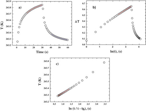
where m₀ is the ambient temperature during heating, which could be influenced by the contact resistance and heating elements adjacent to the temperature sensor inside the needle; m₂ is the background temperature drift rate; m₃ is the slope of the linear relationship between the temperature and the logarithm of the time; and t is the time. The following model was applied to the tempering process:

(2)

The thermal conductivity was calculated using the following equation:

(3)

Effect of the fitting method

Fig. 1a shows the best nonlinear least squares analysis (NLLSA) fits of Eq. (1) (red) and (2) (blue) to the data, whereas Figs. 1b and 1c show the linear least squares analysis (LLSA) fits obtained for Eq. (1), by modelling with the ∆T = T_i – T vs. ln(t) data with ∆T = A + B ln(t), and for Eq. (2), by modelling the T vs. ln(t/(t – t_h)) data with T = A + B ln(t/(t – t_h)), respectively.

It should be noted that in this work, the initial time data were ignored, and only the final 2/3 of the data collected during heating and tempering were used because Eqs. (1) and (2) are long-term approximations of exponential integral equations. Furthermore, undesirable contact resistance effects mainly appear in the initial data. It should also be noted that neglecting the initial time data during fitting results in correlation coefficients (R²) of greater than 0.9997 for Eq. (1) and 0.9995 for Eq. (2) for all t_h values studied.

Table 2 lists the k values for the different t_h values estimated by both the NLLSA and LLSA methods. For a given heating time t_h, the k values obtained by the two fitting methods are similar. Because LLSA generally gives reliable results, whereas NLLSA can give a wide range of results depending on the initial estimates used to solve Eqs. (1) and (2), the thermal conductivities were calculated using the LLSA method in the following sections.

Table 2. Thermal conductivity, k, from the NLLSA and the LLSA of Eqs. 1 and 2 at different heating times, t_h.

	k	k	k	k
Heating time (min)	(NLLSA Eq. 1)	(LLSA Eq. 1)	(NLLSA Eq. 2)	(LLSA Eq. 2)
1	1.81 ± 0.03	2.009 ± 0.04	1.80 ± 0.02	1.777 ± 0.005
2	2.06 ± 0.01	2.113 ± 0.002	1.903 ± 0.03	2.0281 ± 0.006
5	2.13 ± 0.02	2.271 ± 0.02	2.20 ± 0.02	2.155 ± 0.004
10	2.39 ± 0.03	2.372 ± 0.02	2.31 ± 0.02	2.024 ± 0.0007

Effect of the heating time

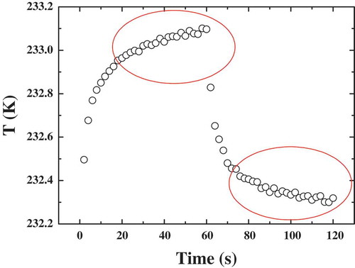
For each ice temperature, different heating times were employed in the following order: t_h = 1, 2, 3, 5, 10, 5, 2, and 1 min. The obtained k values are listed in Table 3. Over the entire temperature range studied, the thermal conductivity increases as t_h is increased from 1 to 5 min and then remains nearly constant within the error as t_h is increased from 5 min to 10 min. Furthermore, a significant hysteresis between the k values obtained before and after heating for 10 min is observed, i.e., the k values determined after the t_h = 10 min measurement are always higher than those determined before that measurement. Table 3 also shows the error for each measurement. The k-error decreases with increasing t_h. However, the k-errors of the measurements at −40°C are high (k-error > 0.01), as is the k-error of the measurement at −30°C with t_h = 1 min. These high errors might be due to the lower accuracy of the detection device at very low temperatures. Figure 2 shows the temperature vs. time data for ice at −40°C with t_h = 2 min. The temperature accuracy for this sample is higher than that for the sample at −10°C with t_h = 2 min during the last two-thirds of the heating and tempering processes (see Fig. 1a). The error in the measurements performed at −5°C is also quite high, possibly due to the concave shape of the temperature vs. time data curves when the heating time was short (data not shown). Therefore, a heating time of 5 min is determined to be the optimal heating time for this system.

Table 3. Thermal conductivity, k, of solid water (ice) at temperatures ranging from −40 to −5 ºC obtained by using different heating time.

Heating rate	k	k-error
−5 ºC
1	1.932	0.0096
2	2.076	0.107
5	2.25	0.0077
10	2.197	0.0044
5	2.198	0.0051
2	2.077	0.0051
−10 ºC
1	1.962	0.0046
2	2.077	0.0036
5	2.222	0.0037
10	2.217	0.0027
5	2.219	0.0031
2	2.091	0.0043
1	1.973	0.0043
−30 ºC
1	1.514	0.12
2	2.278	0.0089
5	2.606	0.0079
10	2.578	0.0073
5	2.537	0.0096
2	2.291	0.0089
1	2.038	0.0573
−40 ºC
1	1.919	0.013
2	2.412	0.0688
5	2.754	0.0388
10	2.591	0.0388
5	2.663	0.359
2	2.469	0.219
1	2.342	0.0573

Figure 2. Temperature vs. time data obtained at −40 °C with t_h = 2 min.

Thermal conductivity of ice prepared by different freezing processes as a function of temperature

Figure 3 shows the thermal conductivities of the ice prepared by slow freezing at –5°C, –10°C, –20°C, –30°C, and –40°C obtained using a heating time of 5 min and LLSA to solve both Eqs. (1) and (2). The results show that k decreases with increasing temperature, in agreement with the findings of Klinbun and Rattanadecho’s study of frozen food.^[27] In this work, k depends linearly on the temperature, increasing by approximately 24% as the temperature is increased from −10°C to −40°C. The data can be fitted by the following equation: k = −0.0176 + 2.0526 T, which is consistent with the results of Choi and Okos^[1] but differs significantly from those of other researchers^[2–9] (see Table 1).

Figure 3. Experimental thermal conductivities of ice reported in the literature and obtained for the different freezing processes in this study.

Figure 3 also compares the thermal conductivities of the ice prepared by fast and slow freezing measured at −20°C (2.64 ± 0.06 W/(m·K) vs. 2.41 ± 0.03 W/(m·K)). Clearly, as the freezing rate increases, the k value increases significantly, by approximately 10%. To appreciate the significance of this difference in the thermal conductivity, it should be noted that it is equivalent to the difference observed when the thermal conductivity is measured at temperatures varying by nearly 15°C (see Fig. 3).

Because the thermal conductivity measured at a given temperature depends on the freezing rate, this property could be used to distinguish between high-quality (fast) and low-quality (slow) freezing processes. Therefore, thermal conductivity measurements might be a promising method for ascertaining how quickly a food product was frozen, although this property must be evaluated for each food^[28] to extend its application.

Ice prepared from aerated and non-aerated water

The thermal conductivities of the ice samples prepared from aerated and non-aerated water measured at –20°C (2.39 ± 0.08 W/(m·K) vs. 2.48 ± 0.06 W/(m·K)) are the same within the error (see Fig. 3), indicating that the dissolved gas concentration of the water does not affect the thermal conductivity of ice.

Ice prepared in the presence of a magnetic field

The thermal conductivities of the ice samples prepared by the 0% CAS and 50% CAS air-blast freezing methods measured at −29°C are both 2.75 ± 0.03 W/(m·K) (see Fig. 3). These results reveal that freezing water in the presence of an AMF does not affect the thermal conductivity of the resulting ice. It should be noted that the k values of the ice prepared in the presence of an AMF are higher than those of the samples prepared by slow freezing. These results can be explained by the fact that the freezing rate was higher in the AMF experiments because the temperature of the air-blast freezer was −50°C during the freezing process.

To our knowledge, the thermal conductivity of ice prepared in the presence of an AMF has not been previously reported. Instead, other related thermal properties of ice or other systems have been measured and used to validate the results, leading to conflicting reports of the effects of AMF freezing in the literature. Zhao et al.^[29] measured the freezing curves of deionized water under a static magnetic field and found that applying a low field intensity ( < 50 mT) did not significantly affect the nucleation temperature and phase transition time. Watanabe et al.^[28] used differential thermal analysis to demonstrate that a weak AMF did not influence the temperature history during pure water freezing. Similar results were reported in studies of several food products^[30,31] that were frozen in the presence and absence of an AMF (0.5 mT/50 Hz) or under nuclear magnetic resonance conditions (static magnetic field of 20 mT, electromagnetic wave frequency of 1 MHz, AMF of 0.12 mT). In these studies, no significant effects of the applied AMF on the degree of supercooling or the freezing times were observed. Furthermore, James et al.^[32] found that varying the AMF ( ≤ 0.418 mT) had little effect on the freezing curve characteristics for garlic bulbs. These results are consistent with those presented in this work. In contrast, Ehrlich et al.^[33] showed that the k value directly impacts the heat transfer in frozen solutions. Moreover, Mok et al.^[34] treated chicken breast samples with a combination of pulsed electric fields and an AMF to achieve a supercooled state at −6.5°C, in contrast to the partially frozen state of the control samples at this temperature.

Conclusions

In this work, a commercial needle probe was used to measure the thermal conductivity k of ice in the temperature range of −5 to −40°C. The results indicate that the measurement protocol affects the k value and therefore could be a source of the conflicting k values of ice reported in the literature. Accordingly, the measurement parameters, such as the heating time and data fitting method, must be optimized to obtain reliable results. These parameters were optimized in this work and then used to determine the thermal conductivities of ice samples prepared by slow freezing at −5, −10, −20, –30 and −40°C. The results are consistent with those of Chio and Okos^[1] but differ from those reported by other researchers.^[2–9]

In addition, the effects of different factors, including the freezing rate, presence of dissolved gasses in the water and presence of a magnetic field during freezing, on the thermal conductivity of ice were studied.

The results show that the presence of dissolved gasses in the water (i.e., impurities) and the presence of an AMF during freezing do not affect the thermal conductivity of ice. However, the freezing rate can significantly affect the k value and could therefore be a source of the discrepancies in the literature values. Moreover, the significant difference in the k values of the ice prepared at different freezing rates indicates that thermal conductivity measurements could be a valuable tool for traceability purposes. However, additional work is necessary to extend this research to real frozen foods, in which factors such as the composition and structure play an important role. Furthermore, to our knowledge, the k value of a material frozen in the presence of an electromagnetic field is reported for the first time in this work, and the results shed light on some of the conflicting data in the literature.

Funding

This work was supported by the Spanish Ministry of Economy and Competitiveness (MINECO) through project AGL2012-39756-C02-01. A.C. Rodríguez acknowledges a predoctoral contract BES-2013-065942 from MINECO through the National Program for the Promotion of Talent and its Employability (National Sub-Program for Doctors Training).

Additional information

Funding

This work was supported by the Spanish Ministry of Economy and Competitiveness (MINECO) through project AGL2012-39756-C02-01. A.C. Rodríguez acknowledges a predoctoral contract from MINECO through the National Program for the Promotion of Talent and its Employability (National Sub-Program for Doctors Training).

References

- Choi, Y.; Okos, M.R. Food Engineering and Process Applications; Elsevier Applied Science Publishers: London, 1986; 93 pp
- Rabin, Y. The Effect of Temperature-Dependent Thermal Conductivity in Heat Transfer Simulations of Frozen Biomaterials. Cryoletters 2000, 21 3, 163–170.
- van Dusen, M.S.; Thermal Conductivity of Non-Metallic Solids. In International Tables of Numerical Data: Physics, Chemisty and Technology; Ed., Washburn, E.W.; McGraw Hill: New York USA, 1929; 216 pp.
- Ratcliffe, E.H. The Thermal Conductivity of Ice New Data on the Temperature Coefficient. Philosophical Magazine 1962, 7, 1197–1203.
- Alexiades, V.; Solomon, A.D. Mathematical Modeling of Melting and Freezing Processes; Hemisphere Publishing: Wasshington, 1993; 65 pp
- Lunardini, V.J. Heat Transfer in Cold Climates; Van Nostrand Reinhold: New York, 1981; 309 pp
- Waite, W.F.; Gilbert, L.Y.; Winters, W.J.; Mason, D.H. Estimating Thermal Diffusivity and Specific Heat from Needle Probe Thermal Conductivity Data. Review of Scientific Instruments 2006, 77, 044904.
- Jakob, M.; Erk, S. Warmedehnung des Eises zwischen Zeitschr. F. Techn. Physik. 1928, 10, 623–624.
- Dean, J.W.; Timmerhous, K.D. Thermal Conductivity of Solid Η2O and D2O at Low Temperature. Advances in Cryogenic Engineering 1963, 8, 263–267.
- Otero, L.; Rodríguez, A.; Mateos, P.; Sanz, P.D. Effects of Magnetic Fields on Freezing: Application to Biological Products. Comprehensive Reviews in Food Science and Food Safety 2016, 15 3, 646–667.
- O’Brien, F.J.; Harley, B.A.; Yannas, I.V.; Gibson, L. Influence of Freezing Rate on Pore Structure in Freeze-Dried Collagen-Gag Scaffolds. Biomaterials 2004, 25 6, 1077–1086.
- Songsaeng, S.; Sophanodora, P.; Kaewsrithong, J.; Ohshima, T. Quality Changes in Oyster (Crassostrea belcheri) during Frozen Storage as Affected by Freezing and Antioxidant. Food Chemistry 2010, 123 2, 286–290.
- Woo, M.W.; Mujumdar, A.S. Effects of Electric and Magnetic Field on Freezing and Possible Relevance in Freeze Drying. Drying Technology 2010, 28 4, 433–443.
- Dalvi-Isfahan, M.; Hamdami, N.; Xanthakis, E.; Le-Bail, A. Review on the Control of Ice Nucleation by Ultrasound Waves, Electric and Magnetic Fields. Journal Food Engineering 2017, 195, 222–234.
- Turgut, A. A Study on Hot Wire Method of Measuring Thermal Conductivity, pHD, 2004, İZMİR.
- Tocci, A.M.; Flores, E.S.E.; Mascheroni, R.H. Enthalpy, Heat Capacity and Thermal Conductivity of Boneless Mutton between – 40°C and + 40°C. Food Science and Technology 1997, 30, 184–191.
- Hsieh, H. The Thermal Conductivity Measurements with a Thermal Probe in the Presence of External Sources; M.S. Georgia Institute of Technology,Atlanta, EE. UU, 1983.
- Lentz, C.P. Thermal Conductivity of Meats, Fats, Gelatin Gels and Ice. Food Technology 1961, 15, 243–247.
- Pham, Q.T.; Willix, J. Thermal Conductivity of Fresh Lamb Meat, Offals and Fat in the Range −40 to +30°C: Measurements and Correlations. Journal of Food Science 1989, 54, 508–515.
- Miller, H.L.; Sunderland, E. Thermal Conductivity of Beef. Food Technology 1963, 17, 490–492.
- Hill, J.E.; Leitman, J.D.; Sunderland, J.E. Thermal Conductivity of Various Meat. Food Technology 1967, 21, 1143–1148.
- Woolf, R.; Sibbitt, W.L. Thermal Conductivity of Liquids. Industrial & Engineering Chemistry 1954, 46, 1947–1952.
- Gentzlerand, G.L.; Schmidt, F.W. Effect of Bound Water in the Freeze-Drying Process. Journal of Food Science 1972, 37, 554–557.
- Wang, D.Q.; Kolbe, E. Thermal Conductivity of Surimi Measurement and Modeling. Journal of Food Science 1990, 55, 1217–1221.
- Sweat, V.E.; Haugh, C.G.; Stadelman, W.J. Thermal Conductivity of Chicken Meat at Temperatures between −75 and 20°C. Journal Food Sciences 1973, 38, 158–160.
- Pongsawatmanit, R.; Miyawaki, O.; Yano, T. Measurement of the Thermal Conductivity of Unfrozen and Frozen Food Materials by a Steady State Method with Coaxial Dual-Cylinder Apparatus. Bioscience, Biotechnology Biochemical 1993, 57 7, 1072–1076.
- Klinbun, W.; Rattanadecho, P. An Investigation of the Dielectric and Thermal Properties of Frozen Foods over a Temperature from −18 to 80°C. International Journal of Food Properties 2017, 20 2, 455–464.
- Seetapan, N.; Limparyoon, N.; Fuongfuchat, A.; Gamonpilas, C.; Methacanon, P. Effect of Freezing Rate and Starch Granular Morphology on Ice Formation and Non-Freezable Water Content of Flour and Starch Gels. International Journal of Food Properties 2016, 19 7, 1616–1630.
- Zhao, H.; Hu, H.; Liu, S.; Han, J. Experimental Study on Freezing of Liquids under Static Magnetic Field. Chinese Journal of Chemical Engineering (in press).
- Watanabe, M.K.; Masuda, K.; Suzuki, T. In 23rd IIR International Congress of Refrigeration, Published by IIF-IIR; Prague, 2011; 21–26.
- Suzuki, T.T.; Masuda, Y.; Watanabe, K.; Shirakashi, M.; Fukuda, R.; Tsuruta, Y.; Yamamoto, T.; Koga, K.; Hiruma, N.; Ichioka, N.; Takai, J. Experimental Investigation of Effectiveness of Magnetic field on Food Freezing Process. Transactions of the Japan Society of Refrigerating and Air Conditioning Engineers 2009, 26 4, 371–386.
- James, C.; Reitz, B.; James, S.J. The Freezing Characteristics of Garlic Bulbs (Allium sativum L.) Frozen Conventionally or with the Assistance of an Oscillating Weak Magnetic Field. Food and bioprocess technology 2015, 8 3, 702–708.
- Ehrlich, L.; Feig, J.S.G.; Schiffres, S.; Malen, J.; Rabin, Y.; Rubinsky, B. Large Thermal Conductivity Differences between the Crystalline and Vitrified States of DMSO with Applications to Cryopreservation. PLoS One 2015, 10 5, e0125862.
- Mok, J.H.; Her, J.-Y.; Kang, T.; Hoptowit, R.; Jun, S. Effects of Pulsed Electric Field (PEF) and Oscillating Magnetic Field (OMF) Combination Technology on the Extension of Supercooling for Chicken Breasts. Journal of Food Engineering 2017, 196, 27–35.