Nondestructive determination of soluble solids content of persimmons by using dielectric spectroscopy

ABSTRACT

To explore the feasibility of dielectric spectroscopy in predicting soluble solids content (SSC) of persimmons during postharvest storage period, the dielectric constant spectra and dielectric loss factor spectra of 105 ‘Shui’ persimmons were measured from 20 MHz to 4500 MHz. Based on the joint x-y distances algorithm, the persimmon samples were divided into two sets: 70 samples in calibration set and 35 samples in prediction set. One hundred and seventy-four, 14, and 24 variables were extracted as characteristic variables from full dielectric spectra (FS) by uninformative variables elimination (UVE), successive projection algorithm (SPA), and competitive adaptive reweighted sampling (CARS), respectively. Partial least squares (PLS) and least squares support vector machine (LSSVM) were applied to build SSC prediction models using FS and characteristic variables extracted by UVE, SPA, and CARS. The results indicated that LSSVM models offered better performance than PLS models at same input variables. CARS-LSSVM had the best SSC determination performance with the correlation coefficient and root-mean-square error of prediction set of 0.970 and 0.494°Brix. This study indicates that dielectric spectroscopy technique combined with characteristic variables selection methods is promising for determining SSC of persimmons.

KEYWORDS:

• Persimmons
• Dielectric spectroscopy technique
• Soluble solids content
• Characteristic variables selection
• Models

Introduction

Persimmon (Diospyros kaki Thunb.), an important commercial fruit crop, is planted widely in Asian countries and in other regions of the world. The production of persimmon fruits in the world reached 4,637,357 t in 2013, with an upward trend since 1991. China is one of the major countries in planting persimmons. It was reported that Chinese production of persimmon fruits in 2013 reached 3,618,823 t.^[1] The persimmon fruit is a nutritionally beneficial fruit which contains large amounts of sugars, vitamin C, carotenoids, and polyphenols in the fresh fruits.^[2] Although persimmons can be used to produce dried persimmon, persimmon vinegar, alcohol, and beverage, etc, fresh-eat persimmons are still the main products in persimmon consumption. Persimmons are usually sorted manually or automatically by their external quality features, such as size, shape, and color. However, sweetness, the main quality attribute of persimmons, directly influences the customers’ purchasing decision. The sweetness of fruit could be evaluated by soluble solids content (SSC), which is mostly sugar. Generally, SSC is measured with an Abbe refractometer or digital refractometer on juice extracted from the fruit pulp. These methods can obtain relatively accurate results, but they are inefficient and destructive. Therefore, it is essential to develop a fast and nondestructive technique to measure the SSC of persimmons for producers, processors, and distributors.

At present, visible/near-infrared spectroscopy technique has been applied to nondestructively predict SSC of persimmons.^[3–5] However, the persimmon samples used in these studies were obtained from only one orchard. The more origins of samples used for modeling is helpful to improve the robustness of the models. Like visible/near-infrared spectroscopy, dielectric spectroscopy, which describes permittivities over a wide frequency range, is also a fast, easy, and nondestructive technique. Dielectric spectroscopy technique has been successfully applied to predict SSC of various fruits such as apples,^[6] honeydew melon,^[7] peaches,^[8] and watermelons.^[9,10] These researches have indicated that dielectric spectroscopy is potential to measure the SSC of fruits. However, no study has been reported on using dielectric spectroscopy to determine the SSC of persimmons. It is interested to study whether the dielectric spectroscopy has potential in nondestructively determining the SSC of fresh persimmons.

Usually, noise from environment and instrumental sources are contained in the full spectra. When the full spectra are applied on on-line detection objective, the models built based on the amount of spectra is unstable and unapplicable.^[11] To overcome this problem, characteristic variables selection methods are usually applied to reduce the dimension of variables by selecting some indispensable and useful variables, usually called characteristic variables. Several studies have shown that characteristic variables selected using chemometric methods was helpful to improve the predictive capability of multivariate calibration models.^[12–14]

In this study, dielectric spectroscopy technique combined with characteristic variables selection approaches was applied to determine the SSC of persimmons during postharvest storage. The main objectives of this research were (1) to extract some characteristic dielectric variables that contain enough useful information by using different characteristic variables selection methods; (2) to build different models for determining SSC of persimmons originated from different orchards; and (3) to evaluate the potential of dielectric spectroscopy in nondestructively determining SSC of persimmons.

Materials and methods

Fruit samples

Persimmons, variety ‘Shui’, a common persimmon cultivar in Northwest China, were picked from three different orchards, located at 34º21′ north latitude, 108º10′ east longitude, and altitudes from 500 m to 950 m, in Yangling, Shaanxi Province, China on 30th September 2015. The persimmons were stored in polyethylene bags with air holes at room temperature (24 ± 2°C). The experiments were done at 5-day interval until the persimmons became a little soft and the SSC measurement was conducted difficultly. Finally, the experiment continued 35 days. The firmness of the used persimmons was 11.2 ± 1.8 kg/cm² at the beginning of experiment, and it was 2.1 ± 0.4 kg/cm² at the end of the experiment. At each experiment, 15 intact persimmons were taken for measurement. Totally, 105 persimmons were used in this research, including 35 persimmons from each orchard. The diameters of all used persimmons were measured with an electronic caliper (Star Precision Instruments Co. LTD., Jiangsu, China) with a precision of 0.1 mm. The diameter of persimmons changed from 55.4 to 72.6 mm, with a mean of 65.1 mm and a standard deviation of 3.4 mm.

Dielectric spectra acquisition

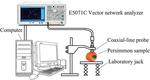
The schematic diagram of the equipment applied to acquire dielectric spectra of persimmons is shown in Figure 1. It was made up of an E5071C vector network analyzer, an 85070E-020 open-ended coaxial-line probe, a N6314A coaxial cable (Agilent Technologies, Penang, Malaysia), a laboratory jack, and a computer. The dielectric properties are represented by the permittivity ε* = ε’-jε’’, here the real part ε’ and the imaginary part ε’’ refer to the dielectric constant and the dielectric loss factor, respectively. The two parameters were measured by computing the reflection coefficient between the persimmon samples and the coaxial-line probe. In this research, 201 dielectric variables were measured in the frequency range of 20–4,500 MHz for both ε’ and ε’’. The 201 variables of ε’ were numbered from 1 to 201, and the 201 variables of ε’’ were numbered from 202 to 402 with the increasing frequency.

Figure 1. The schematic diagram of the dielectric spectra measurement system.

Dielectric properties and internal qualities measurement

The E5071C network analyzer was powered on for more than 1 h, then calibrated in sequence at the port used for the permittivity measurements. The 85070E-020 coaxial-line probe was calibrated by air, short-circuit, and 25°C deionized water. A test was made on 25°C deionized water to verify whether accurate permittivity values were acquired. The dielectric properties measurement of fresh persimmons were made at room temperature (24 ± 2°C). Three points at 120º apart around the equatorial region of the fruit were measured for each persimmon. After dielectric spectra of persimmons were obtained, the SSC of juice extracted from the persimmon tissue was measured with a digital reflectometer (Model PR101a, Atago Co. Ltd., Tokyo, Japan). The means of three measurements on ε’, ε’’, and three SSC readings for each persimmon were calculated as the reference value of SSC.

Sample division method

A reasonable sample division is helpful to enhance the robustness and prediction accuracy of models. In this research, the joint x–y distances (SPXY) algorithm was applied for sample partitioning. The SPXY sample division is an algorithm developed from classic Kennard–Stone (KS) method. In KS algorithm, only the differences of x (instrumental responses) space were considered. SPXY extends the KS method by considering the Euclidean distance of both x and y (target attributes).^[15] Euclidean distance d_x(p,q) is calculated as:

(1)

where x_p(j) and x_q(j) represent the response of the j-th dielectric spectral variable of persimmons p and q, respectively. J represents the number of full dielectric spectral variables, and N represents the number of persimmons. In this research, the value of J and N is 402 and 105, respectively. The function d_y(p,q) for samples p and q can be calculated in the following:

(2)

where y_p and y_q denotes the SSC of persimmon samples p and q, respectively. The function d_xy(p,q) could be computed as:

(3)

Some samples can then be divided into the calibration set according to the value of d_xy (p,q). The remaining samples are divided into the prediction set.

Characteristic variables selection methods

Characteristic variables selection is often applied for reducing the complexity of models, enhancing the robustness of models, and improving prediction accuracy of models. In this study, three effective methods were used to select characteristic variables that contain most of the important information for the SSC prediction of persimmons.

Uninformative variables elimination

The uninformative variables elimination (UVE) method is an algorithm for choosing vital variables using stability analysis of partial least squares (PLS).^[16] It aims to remove the variables that contain less useful information for modeling than random signal. When executing UVE, random noise is manually added to spectral variable set to eliminate the variables which provide less useful information than random noise. A model established using characteristic variables chosen by UVE could avoid the problem of over fitting and improve the models’ predictive ability. More detailed information on the algorithm can be found in other literature.^[17]

Successive projections algorithm

Successive projection algorithm (SPA) was put forward to choose characteristic variables for building models by Araújo et al.^[18] It adopts projection operations to find out some representative variables with minimal collinearity. The main procedures of SPA are summarized in the following: (1) set the largest number of representative variables K to be chosen in a M-dimensions (here M presents total number of full spectral variables) space; (2) the vector with minimal collinearity is chosen and used as the new initial vector in an orthogonal sub-space; (3) keep the iteration until the number of variables gets to K. At present, the variable selection method has been used to choose characteristic variables in NIR spectroscopy technique^[19,20] and dielectric spectroscopy technique.^[21] More details about the method was described by Araújo et al.^[18]

Competitive adaptive reweighted sampling

Competitive adaptive reweighted sampling (CARS), proposed by Li et al.,^[22] is an algorithm for choosing a few representative variables by removing insignificance variables in stepwise way. Main procedures of CARS are summarized as follows: Firstly, Monte Carlo algorithm is executed to determine the samples for building PLS model. The regression coefficients of PLS model would be considered as the evaluation index. Secondly, the exponentially decreasing function is applied to select important variables with higher PLS regression coefficients values. Then, adaptive reweighted sampling is used to choose relative useful variables randomly. The remained variables are used for next evaluation loop. Finally, the subset with the minimum root mean square error of cross validation (RMSECV) is selected as the optimal variables combination for the subsequent modeling. More details about CARS could be found elsewhere.^[22] Up to now, CARS has been successfully used in characteristic variables selection and has obtained excellent determination performance.^[23–25]

Modeling methods

In this research, a linear modeling method, i.e., partial least squares (PLS), and a nonlinear modeling method, i.e., least squares support vector machine (LSSVM), were applied to develop SSC determination models of persimmons.

Partial least squares

PLS is one of the most popular multi-analysis approaches which are insensitive to collinear data. The objective of PLS algorithm is to project original spectral data onto a small number of latent variables (LVs). The LVs that contain most information of the original spectral data will be used for the next modeling. The number of LVs is the most important parameter for modeling because the selected LVs are employed as the input of PLS.^[26] A reasonable choice for the number of LVs could avoid the problems of over fitting or under fitting in the process of establishing a PLS model.

Least squares support vector machine

Support vector machines (SVMs) are powerful and widely used algorithms for data classification and regression. It is carried out by using statistical learning theory. Risk minimization principle is employed to avoid over fitting or under fitting problem in the modeling. However, the matrix size of the quadratic programming is directly proportional to the number of modeling set. This makes the standard quadratic programming difficult to be applied for high-dimensional dataset.^[27] Therefore, the least squares support vector machine (LSSVM) was proposed as a modified version of SVM to simplify the algorithm.^[28] More details about LSSVM algorithm could be found elsewhere.^[29]

Model assessment

In this study, correlation coefficient of calibration set (R_c), correlation coefficient of prediction set (R_p), root-mean-square error of calibration set (RMSEC), and root-mean-square error of prediction set (RMSEP) were chosen as the evaluation index of the models. They are calculated as follows:

(4)

(5)

(6)

(7)

where represents the predicted SSC value of the i-th persimmon. y_i represents the measured SSC value of the i-th persimmon. y_c represents to the mean SSC value of the calibration set, and y_p represents the mean SSC value of prediction set. n_c and n_p refer to the number of samples in the calibration set and the prediction set, respectively. Generally, a model with good performance should have high values of R_c and R_p, and low values of RMSEC and RMSEP.

In addition to the above evaluation indices, residual predictive deviation (RPD), defined as the ratio of the standard deviation of the internal quality attribute in prediction set to RMSEP, was chosen as an evaluation index of the prediction ability of a model. Generally, a RPD value lower than 1.5 means poor prediction, a value between 1.5 and 2.0 indicates that it could discriminate low from high values of the internal quality attribute, a value between 2.0 and 2.5 means that coarse predictions are possible, and a value between 2.5 and 3.0 or above 3.0 represents the model have a good or excellent prediction ability.^[30]

Software

In addition to the above-described 85070E for acquiring dielectric spectra of persimmons, Matlab R2013a (Math Works, Massachusetts, USA) was applied to accomplish statistic analysis of SSC, to select characteristic variables, and to establish SSC determination models of persimmons.

Results and discussion

Dielectric spectra and SSC of persimmons

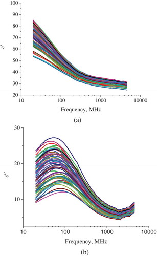
Figure 2 shows the original dielectric spectra of the 105 persimmon samples at 201 discrete frequencies in the range of 20–4500 MHz. It can be seen that all persimmon samples had similar spectra of ε’ and ε’’. The ε’ decreased monotonically as frequency increased. Especially in the range of 20–200 MHz, the spectra of ε’ declined sharply with increasing frequency. The ε’’ firstly increased to a maximum at about 50–80 MHz, then it decreased to a minimum at about 2000 MHz before increasing. The dielectric loss factor behavior of fresh fruits was also found in apples and peaches in the range of 20–4500 MHz.^[31,32] The overriding dielectric relaxation behavior of dielectric loss factor might be caused by bound water and Maxwell-Wagner relaxations.^[33]

Figure 2. The spectra of dielectric constant (a) and dielectric loss factor (b) of intact persimmons over the frequency from 20 to 4500 MHz.

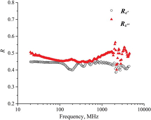
The statistics for the SSC values of all used persimmons are shown in Table 1. It could be seen that the SSC of persimmons changed from 14.2 to 22.8 ºBrix, with a mean of 18.5 ºBrix and a standard deviation of 2.1 ºBrix. In order to know whether the permittivities (ε’ or ε’’) at a certain individual frequency had correlation with SSC of persimmons, their linear relationship y = a*SSC+b, where y presents ε’ or ε’’ at a single frequency, was calculated. The linear correlation coefficient between the permittivities and SSC is shown in Figure 3. It can be seen that the linear correlation coefficient was lower than 0.45 and 0.56 for ε’ and ε’’, respectively. This indicated that it was impossible to determine the SSC of persimmons using a single permittivity value. Therefore, the dielectric spectra combined with chemometric methods were applied to build prediction models of SSC for persimmons.

Table 1. The statistics for the SSC values of persimmons.

Sample sets	Amount of samples	Min., ºBrix	Max., ºBrix	mean ± SD*, ºBrix
All samples	105	14.2	22.8	18.5 ± 2.1
Calibration set	70	14.2	22.8	18.7 ± 2.1
Prediction set	35	14.3	22.5	18.2 ± 2.0

* SD represents standard deviation.

Figure 3. Linear correlation between the permittivities and SSC of persimmons over the frequency range of 20–4500 MHz.

Sample division

The analysis of variance on SSC of 105 persimmons from three orchards was done previously. The results showed that the SSC values of persimmons from three different orchards had not significant differences at the significance level of 5%. Therefore, all the samples from each orchard were put together for sample division in this study. Based on the SPXY algorithm, 105 persimmon samples were divided into two sets: 70 persimmons in calibration set and 35 persimmons in prediction set. The SSC of persimmons in calibration and prediction sets shows that the minimum value of SSC in calibration set was smaller than that in prediction set, and the maximum value of SSC in calibration set was larger than that in prediction set. This means the samples used for modeling included a broader range than the samples used for verifying models, which was conducive to building a reasonable and powerful calibration model.

Selection of characteristic variables

Characteristic variables selected by UVE

The variable selection process by UVE is influenced by the number of LVs when building a PLS model. In this research, the optimal number of LVs was chosen according to the minimum RMSECV. Figure 4 shows the changed RMSECV value with the increasing number of LVs. It could be seen that when 21 LVs were used for modeling, the RMSECV was the smallest (0.742°Brix).

Figure 4. The calculated RMSECV at different number of LVs from 1 to 30 in PLS of UVE. “□” represents the point at which the final number of latent variables was selected.

Figure 5 shows the stability distribution of each variable when UVE algorithm was performed with 21 LVs. The full dielectric spectra (FS) were at the left of the vertical line, and the same number of random variables were at the right side. The two horizontal lines represented the cutoff threshold (±6.7125) of UVE algorithm. The FS whose stabilities were within the cutoff threshold were regarded as uninformative variables. Finally, 174 characteristic variables, including 76 for ε’ and 98 for ε’’, were extracted based on UVE method. The number of extracted characteristic variables was 43.3% of the 402 variables in the FS. All the 174 dielectric variables chosen by UVE were shown in Figure 6.

Figure 5. Stability of each dielectric variable in the dielectric spectra for predication by UVE. Two horizontal dashed lines show the lower and upper cutoff.

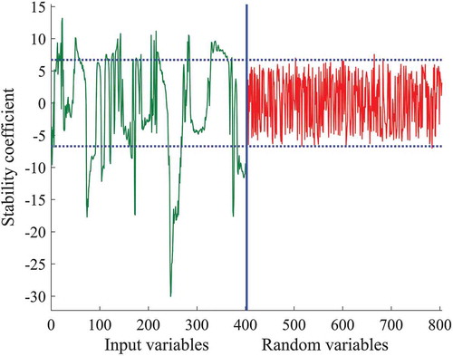
Figure 6. The distribution of selected characteristic variables using UVE over the full dielectric spectra of dielectric constant (a) and loss factor (b) from 20 to 4500 MHz.

Characteristic variables selected by SPA

SPA algorithm was implemented by comparing the RMSECV values at different variable numbers from 1 to 20. The change of RMSECV values with the number of variables selected by SPA is shown in Figure 7. It shows that when the variable number was 14, the RMSECV reached the minimum (0.667°Brix). Therefore, 14 variables were selected as characteristic variables, including 5 variables of ε’ at 27.9, 130.7, 199.6, 2806.3, and 4405.9 MHz, and 9 variables of ε’’ at 20.0, 32.2, 73.9, 461.7, 2070.7, 2234.9, 3465.0, 4123.6, and 4500.0 MHz. Among them, the characteristic variables of ε’ near 27.9, 130.7, and 4405.9 MHz, and variables of ε’’ near 20.0 and 2234.9 MHz were also found in determining the SSC of peaches^[8] and Korla fragrant pears.^[34] It indicates that these frequencies might be related to the SSC of fruits. The amount of selected characteristic variables by SPA was only 3.5% of the 402 variables in the FS.

Figure 7. Changed RMSECV with the number of variables included in SPA. “□” represents the point at which the final number of variables was selected.

Characteristic variables selected by CARS

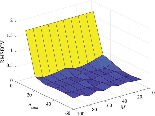
When executing CARS program, three critical parameters were required to be determined. They are sampling number n_sam, repeated sampling number M and calculation loops number N. In general, CARS method can acquire a better performance when the parameter of N takes 100.^[35,36] In order to obtain an optimal pair of n_sam and M, calculations of CARS based on different pairs of n_sam and M were made with a fixed N of 100. The n_sam was set from 10 to 60 with an interval of 10, while the M was set from 10 to 100 with an interval of 10. Every pair of n_sam and M was optimized by 5-fold cross-validation in PLS model calibration to calculate the minimum of RMSECV for the optimal subset of dielectric variables. The calculated RMSECV at different n_sam and M is shown in Figure 8. The figure indicates that the values of RMSECV were influenced by n_sam and M, and the lowest RMSECV (0.295°Brix) was obtained when the value of n_sam and M was 60 and 80. Therefore, the value of n_sam and M were set to 60 and 80, respectively, in the following study.

Figure 8. The optimization of parameters n_sam and M in CARS calculation.

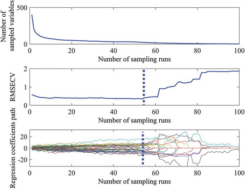
After selecting the parameters, the CARS method was implemented for extracting characteristic variables. Because the samples for developing PLS models were chosen randomly in every sampling run of the CARS, the CARS algorithm was run 100 times to obtain the minimum RMSECV. Figure 9 shows the executing processes of CARS. With the increasing number of sampling, the number of sampled dielectric variables in the subset decreased (Figure 9a). The optimal variable subset was chosen according to the minimum RMSECV of dielectric variable subsets, which was shown in Figure 9b. It showed that with the increasing number of sampling runs, the RMSECV decreased slowly until it arrived at the minimum due to elimination of some useless dielectric variables. Then, it increased rapidly because of elimination of too many important dielectric variables that contain useful information. The regression coefficient path of each variable in the process of CARS with the number of sampling runs changed from 1 to 100 is shown in Figure 9c. The subset which obtained the minimum RMSECV was marked in a vertical dashed line. It can be seen that the minimum RMSECV was 0.348°Brix when the number of sampling runs was 54 (Figure 9b). There were 24 dielectric variables located at the 54th loop (Figure 9a) in total. Therefore, 24 variables were selected as characteristic variables, including 13 variables of at 25.8, 27.9, 32.2, 34.4, 41.8, 84.6, 163.6, 243.5, 483.3, 494.1, 2453.9, 3841.4, and 3935.4 MHz, and 11 variables of ε’’ at 23.6, 28.6, 30.1, 30.8, 33.7, 40.6, 80.3, 138.0, 321.6, 1141.1, and 2994.5 MHz. Among them, the characteristic variables of ε’ near 27.9 and 243.5 MHz, and variables of ε’’ near 23.6 and 2994.5 MHz were also found in determining the SSC of apples^[32] and Korla fragrant pears.^[34] These frequencies might be related to the SSC of fruits. The amount of selected characteristic variables by CARS was only 6.0% of the 402 variables in the FS.

Figure 9. The changes of the number of sampled variables (a), RMSECV (b), and regression coefficients path of each variable (c) during the calculation of CARS.

Modeling results

PLS determination models

In order to avoid under fitting or over fitting problem in building PLS models, determining a proper amount of LVs is necessary. In this study, the optimal number of LVs was determined according to the minimal value of RMSECV. The determined numbers of LVs when FS and different characteristic variables selected using UVE, SPA, and CARS were used as the input of PLS, respectively, are shown in Table 2.

Table 2. The modeling parameters of PLS and LSSVM.

	PLS	LSSVM
Characteristic variable selection methods	Number of factors	γ	σ^2
FS	18	1474896	191877
UVE	20	1654392	61153
CARS	13	3445894	13852
SPA	13	459816	1997

The SSC prediction performances of PLS at different input variables are shown in Table 3. It shows that the PLS model developed using characteristic variables selected by CARS (CARS-PLS) had the highest R_c (0.994) and the lowest RMSEC (0.223°Brix), meaning CARS-PLS had the best calibration performance. In addition, CARS-PLS also obtained the highest R_p (0.970) and RPD (3.563), and the lowest RMSEP (0.561°Brix), indicating CARS-PLS model also had the best prediction performance. The PLS model developed using characteristic variables chosen by SPA (SPA-PLS) had the lowest R_c (0.969) and R_p (0.934), and the highest RMSEC (0.511°Brix) and RMSEP (0.706°Brix), meaning both the calibration and prediction performance of SPA-PLS were the worst. Among four developed PLS models, the SPA-PLS, whose RPD value was higher than 2.5 and lower than 3.0, had good SSC prediction ability. Other three models, whose RPD value was higher than 3.0, had excellent SSC determination ability.

Table 3. Comparison of modeling results using PLS and LSSVM.

		Calibration set		Prediction set
Modeling methods	Characteristic variables selection methods	Rc	RMSEC, ºBrix	Rp	RMSEP, ºBrix	RPD
PLS	FS	0.982	0.324	0.954	0.651	3.080
	UVE	0.988	0.323	0.968	0.635	3.147
	SPA	0.969	0.511	0.934	0.706	2.830
	CARS	0.994	0.223	0.970	0.561	3.563
LSSVM	FS	0.992	0.294	0.959	0.636	3.143
	UVE	0.993	0.285	0.969	0.624	3.204
	SPA	0.989	0.306	0.946	0.692	2.891
	CARS	0.997	0.161	0.970	0.494	4.047

LSSVM determination models

When using LSSVM, there are two critical problems to be solved, i.e., the suitable kernel function and the optimal kernel parameters. Radial basis function (RBF) kernel was chosen for the execution of LSSVM. RBF is a nonlinear function which is conductive to reduce the complexity of calculation and improve the execution efficiency of the program (Wu et al., 2008). Grid search method and leave one out cross-validation were used to determine the optimal parameters, namely, regularization parameter γ and the RBF kernel function parameter σ². The two parameters were optimized in the range of 10^–4-10⁷ with an increment of 10^–4. At each combination of γ and σ², RMSECV was calculated, and the optimal combination (γ, σ²) was determined based on the smallest RMSECV. The determined optimal values of γ and σ² at different characteristic variables selection methods are listed in Table 2.

The SSC prediction performances of LSSVM at different input variables are listed in Table 3. Table 3 shows that the CARS-LSSVM model had the highest R_c (0.997), R_p (0.970), and RPD (4.047), and the lowest RMSEC (0.161°Brix) and RMSEP (0.494°Brix). This indicates that the CARS-LSSVM model not only had the best calibration performance, but also had the best prediction performance. The LSSVM model developed using selected characteristic variables by SPA (SPA-LSSVM) had the lowest R_c (0.989) and R_p (0.946), and the highest RMSEC (0.306°Brix) and RMSEP (0.692°Brix), meaning it had the worst calibration and prediction performance. The RPD of SPA-LSSVM (2.891) model was between 2.5 and 3.0, presenting the model can predict SSC of persimmons precisely. The FS-LSSVM, UVE-LSSVM and CARS-LSSVM had RPD values higher than 3.0, indicating these models had excellent SSC determination ability.

Comparison

When different characteristic variables selection methods were compared, the results showed that for both PLS and LSSVM models, the CARS methods obtained the best calibration and prediction performances, followed by UVE, FS, and SPA. It indicates that the CARS could extract enough important information from FS. However, the FS not only contained useful information but also included noise. The worst performance of SPA tells that more indispensible and important information was lost during characteristic variables selected using SPA. The better variable selection methods performance of CARS than that of UVE and SPA had also been noticed in other studies.^[22,23,37]

When comparing the SSC determination performance of PLS and LSSVM models, the results showed that the LSSVM models offered better performance at the same characteristic variables selection method. For example, compared between PLS and LSSVM models based on UVE, the values of R_c, RMSEC, R_p, RMSEP, and RPD of UVE-LSSVM and UVE-PLS were 0.993 vs. 0.988, 0.285 ºBrix vs. 0.323 ºBrix, 0.969 vs. 0.968, 0.624 ºBrix vs. 0.635 ºBrix, and 3.204 vs. 3.147, respectively. The better performance of LSSVM than that of PLS was also found in other studies, such as in determining organic acids of plum vinegar,^[38] in predicting the moisture content of prawns,^[39] and in determining the SSC of kiwifruits.^[40] Among 8 developed SSC prediction models, the CARS-LSSVM had the best calibration performance with R_c of 0.997 and RMSEC of 0.161°Brix, and the best prediction performance with R_p of 0.970 and RMSEP of 0.494°Brix. The RPD value of CARS-LSSVM was also the highest (4.047). Therefore, CARS-LSSVM is regarded as the best model for SSC determination of persimmons.

Compared with other reported results for SSC determination of persimmons using near-infrared spectroscopy technique, it was found that the obtained best RMSEP (0.494°Brix) in this study were lower than reported 0.257°Brix by Zhang et al.^[3] and 0.448°Brix by Zhang et al.,^[4] but it was higher than 0.498°Brix reported by Wang et al.^[5] It is worth to mention that the samples used in their studies using near-infrared spectroscopy were obtained from one orchard or purchasing from market with no information about the origin. Although the persimmons used in our study were ‘Shui’ variety only, the samples were picked from three orchards which were cultivated by different owners. The more origins used for modeling, the more difficult it is to improve model performance, but the models have wide range in application. The study shows that dielectric spectroscopy could be used as an alternative method for determining SSC of persimmons.

Conclusion

The potential of dielectric spectroscopy technique in nondestructively determining SSC of persimmons was investigated in this study. By using SPXY algorithm, the 105 persimmon samples were divided into two sets: 70 samples in calibration set and 35 samples in prediction set. One hundred and seventy-four, 14, and 24 variables were selected as characteristic variables by UVE, SPA, and CARS, respectively. The CARS methods had the best calibration and prediction performances for both PLS and LSSVM models. In the comparison of modeling methods, LSSVM models offered better performance than PLS models at same input variables. The best SSC determination model for persimmons was CARS-LSSVM with R_p of 0.970, RMSEP of 0.494°Brix, and RPD of 4.047. This study offers an alternative method for determining SSC of persimmons. The theory of the relationship between SSC and dielectric properties will be studied further.

Additional information

Funding

The authors gratefully acknowledge the financial support provided by National Natural Science Foundation of China (Projects No. 31171720 and No. 31671935).

References

- FAOSTAT Food and Agriculture Organization of the United Nations Statistics Division. 2015. http://www.fao.org/faostat/en/#data/QC (accessed June 21, 2016).
- Jiménez-Sánchez, C.; Lozano-Sánchez, J.; Marti, N.; Saura, D.; Valero, M.; Segura-Carretero, A.; Fernández-Gutiérrez, A. Characterization of Polyphenols, Sugars, and Other Polar Compounds in Persimmon Juices Produced under Different Technologies and Their Assessment in Terms of Compositional Variations. Food Chem. 2015, 182, 282–291. DOI: 10.1016/j.foodchem.2015.03.008.
- Zhang, S.; Zhang, H.; Wang, F.; Zhao, C.; Yang, G. Measurement of Soluble Solid Content in Persimmon Using Visible-Near Infrared Spectroscopy. Trans. Chin. Soc. Agric. Eng. 2009, 25(Supp.2), 345–347 (in Chinese with English abstract).
- Zhang, P.; Li, J.; Meng, X.; Zhang, P.; Wang, B.; Feng, X. Nondestructive Determination of Soluble Solid Content in Mopan Persimmon by Visible and Near-Infrared Diffuse Reflection Spectroscopy. Food Sci. 2011, 32(6), 191–194 (in Chinese with English abstract).
- Wang, D.; Lu, X.; Zhang, P.; Li, J.; Chen, S. Testing of Internal Qualities of Mopan Persimmon in Different Storage by Near-Infrared Spectroscopy. Chin. J. Spectrosc. Lab. 2013, 30(6), 2769–2774 (in Chinese with English abstract).
- Guo, W.; Zhu, X.; Nelson, S. O.; Yue, R.; Liu, H.; Liu, Y. Maturity Effects on Dielectric Properties of Apples from 10 to 4500mhz. LWT-Food Sci. Technol. 2011, 44(1), 224–230. DOI: 10.1016/j.lwt.2010.05.032.
- Nelson, S. O.; Trabelsi, S.; Kays, S. J. Dielectric Spectroscopy of Honeydew Melons from 10 MHz to 1.8 GHz for Quality Sensing. Trans. ASABE 2006, 49(6), 1977–1981. DOI: 10.13031/2013.22278.
- Zhu, X.; Fang, L.; Gu, J.; Guo, W. Feasibility Investigation on Determining Soluble Solids Content of Peaches Using Dielectric Spectra. Food Anal. Methods 2015, 9(6), 1789–1798. DOI: 10.1007/s12161-015-0348-7.
- Nelson, S. O.; Guo, W. C.; Trabelsi, S.; Kays, S. J. Dielectric Properties of Watermelons for Quality Sensing. Meas. Sci. Technol. 2007, 18(7), 1887. DOI: 10.1088/0957-0233/18/7/014.
- Guo, W.; Nelson, S.; Trabelsi, S.; Jkays, S. Radio Frequency(RF) dielectric Properties of Honeydew Melon and Watermelon Juice and Correlations with Sugar Content. Trans. Chin. Soc. Agric. Eng. 2008, 24(5), 289–292.
- Andersen, C. M.; Bro, R. Variable Selection in Regression—A Tutorial. J. Chemom. 2010, 24(11–12), 728–737. DOI: 10.1002/cem.v24.11/12.
- Wu, D.; Sun, D.-W. Potential of Time Series-Hyperspectral Imaging (TS-HSI) for Non-Invasive Determination of Microbial Spoilage of Salmon Flesh. Talanta 2013, 111(13), 39–46. DOI: 10.1016/j.talanta.2013.03.041.
- Cheng, P.; Fan, W.; Xu, Y. Determination of Chinese Liquors from Different Geographic Origins by Combination of Mass Spectrometry and Chemometric Technique. Food Contr. 2014, 35(1), 153–158. DOI: 10.1016/j.foodcont.2013.07.003.
- Huang, L.; Di, W.; Jin, H.; Zhang, J.; Yong, H.; Lou, C. Internal Quality Determination of Fruit with Bumpy Surface Using Visible and near Infrared Spectroscopy and Chemometrics: A Case Study with Mulberry Fruit. Biosystems Eng. 2011, 109(4), 377–384. DOI: 10.1016/j.biosystemseng.2011.05.003.
- Galvão, R. K. H.; Araujo, M. C. U.; José, G. E.; Pontes, M. J. C.; Silva, E. C.; Saldanha, T. C. B. A Method for Calibration and Validation Subset Partitioning. Talanta 2005, 67(4), 736–740. DOI: 10.1016/j.talanta.2005.03.025.
- Cai, W.; Li, Y.; Shao, X. A Variable Selection Method Based on Uninformative Variable Elimination for Multivariate Calibration of Near-Infrared Spectra. Chemometrics Intell. Lab. Syst. 2008, 90(2), 188–194. DOI: 10.1016/j.chemolab.2007.10.001.
- Centner, V.; Massart, D.-L.; deNoord, O. E.; deJong, S.; Vandeginste, B. M.; Sterna, C. Elimination of Uninformative Variables for Multivariate Calibration. Anal. Chem. 1996, 68(21), 3851–3858. DOI: 10.1021/ac960321m.
- Araújo, M. C. U.; Saldanha, T. C. B.; Galvão, R. K. H.; Yoneyama, T.; Chame, H. C.; Visani, V. The Successive Projections Algorithm for Variable Selection in Spectroscopic Multicomponent Analysis. Chemometrics Intell. Lab. Syst. 2001, 57(2), 65–73. DOI: 10.1016/S0169-7439(01)00119-8.
- Liu, D.; Guo, W. Identification of Kiwifruits Treated with Exogenous Plant Growth Regulator Using Near-Infrared Hyperspectral Reflectance Imaging. Food Anal. Methods 2015, 8(1), 164–172. DOI: 10.1007/s12161-014-9885-8.
- Xie, C.; Xu, N.; Shao, Y.; He, Y. Using FT-NIR Spectroscopy Technique to Determine Arginine Content in Fermented Cordyceps Sinensis Mycelium. Spectrochimica Acta . A: Mol. Biomol. Spectrosc. 2015, 149, 971–977. DOI: 10.1016/j.saa.2015.05.028.
- Guo, W.; Fang, L.; Liu, D.; Wang, Z. Determination of Soluble Solids Content and Firmness of Pears during Ripening by Using Dielectric Spectroscopy. Comput. Electron. Agric. 2015, 117, 226–233. DOI: 10.1016/j.compag.2015.08.012.
- Li, H.; Liang, Y.; Xu, Q.; Cao, D. Key Wavelengths Screening Using Competitive Adaptive Reweighted Sampling Method for Multivariate Calibration. Anal. Chim. Acta 2009, 648(1), 77–84. DOI: 10.1016/j.aca.2009.06.046.
- Fan, S.; Huang, W.; Guo, Z.; Zhang, B.; Zhao, C. Prediction of Soluble Solids Content and Firmness of Pears Using Hyperspectral Reflectance Imaging. Food Anal. Methods 2015, 8(8), 1936–1946. DOI: 10.1007/s12161-014-0079-1.
- Tang, G.; Hu, J.; Yan, H.; Zhao, Y.; Xiong, Y.; Min, S. Determination of Active Ingredients in Matrine Aqueous Solutions by Mid-Infrared Spectroscopy and Competitive Adaptive Reweighted Sampling. Optik-International J. Light . Opt. 2015, 127(3), 1405–1407. DOI: 10.1016/j.ijleo.2015.09.139.
- Fan, S.; Zhang, B.; Li, J.; Huang, W.; Wang, C. Effect of Spectrum Measurement Position Variation on the Robustness of NIR Spectroscopy Models for Soluble Solids Content of Apple. Biosystems Eng. 2016, 143(45), 9–19. DOI: 10.1016/j.biosystemseng.2015.12.012.
- Zou, X.; Zhao, J.; Huang, X.; Yanxiao, L. I. Use of FT-NIR Spectrometry in Non-Invasive Measurements of Soluble Solid Contents (SSC) of ‘Fuji’ Apple Based on Different PLS Models. Chemometrics Intell. Lab. Syst. 2007, 87(1), 43–51. DOI: 10.1016/j.chemolab.2006.09.003.
- Chua, K. S.;. Efficient Computations for Large Least Square Support Vector Machine Classifiers. Pattern Recognit. Lett. 2003, 24(1–3), 75–80. DOI: 10.1016/S0167-8655(02)00190-3.
- Suykens, J. A.; Vandewalle, J. Least Squares Support Vector Machine Classifiers. Neural Process. Lett. 1999, 9(3), 293–300. DOI: 10.1023/A:1018628609742.
- Ferrão, M. F.; Godoy, S. C.; Gerbase, A. E.; Mello, C.; Furtado, J. C.; Petzhold, C. L.; Poppi, R. J. Non-Destructive Method for Determination of Hydroxyl Value of Soybean Polyol by LS-SVM Using HATR/FT-IR. Anal. Chim. Acta 2007, 595(1–2), 114–119. DOI: 10.1016/j.aca.2007.02.066.
- Nicolaї, B. M.; Beullens, K.; Bobelyn, E.; Peirs, A.; Saeys, W.; Theron, K. I.; Lammertyn, J. Nondestructive Measurement of Fruit and Vegetable Quality by Means of NIR Spectroscopy: A Review. Postharvest Biol. Technol. 2007, 46(2), 99–118. DOI: 10.1016/j.postharvbio.2007.06.024.
- Zhu, X.; Fang, L.; Gu, J.; Guo, W. Feasibility Investigation on Determining Soluble Solids Content of Peaches Using Dielectric Spectra. Food Anal. Methods 2016, 9(6), 1789–1798. DOI: 10.1007/s12161-015-0348-7.
- Guo, W.; Shang, L.; Zhu, X.; Nelson, S. O. Nondestructive Detection of Soluble Solids Content of Apples from Dielectric Spectra with ANN and Chemometric Methods. Food Bioprocess Technol. 2015, 8(5), 1126–1138. DOI: 10.1007/s11947-015-1477-0.
- Guo, W.; Nelson, S. O.; Trabelsi, S.; Stanley, J. K. Dielectric Properties of Honeydew Melons and Correlation with Quality. J. Microwave Power Electromagn. Energy 2006, 41(2), 44–54. DOI: 10.1080/08327823.2006.11688556.
- Fang, L.; Guo, W. Nondestructive Measurement of Sugar Content and Firmness in Korla Fragrant Pears by Using Their Dielectric Spectra. Mod. Food Sci. Technol. 2016, 32(5), 295–301.
- Jiang, H.; Zhang, H.; Chen, Q.; Mei, C.; Liu, G. Identification of Solid State Fermentation Degree with FT-NIR Spectroscopy: Comparison of Wavelength Variable Selection Methods of CARS and SCARS. Spectrochimica Acta . Mol. Biomol. Spectrosc. 2015, 149, 1–7. DOI: 10.1016/j.saa.2015.04.024.
- Zheng, K.; Li, Q.; Wang, J.; Geng, J.; Cao, P.; Sui, T.; Wang, X.; Du, Y. Stability Competitive Adaptive Reweighted Sampling (SCARS) and Its Applications to Multivariate Calibration of NIR Spectra. Chemometrics Intell. Lab. Syst. 2012, 112(6), 48–54. DOI: 10.1016/j.chemolab.2012.01.002.
- Li, X.; Wang, S.; Shi, W.; Shen, Q. Partial Least Squares Discriminant Analysis Model Based on Variable Selection Applied to Identify the Adulterated Olive Oil. Food Anal. Methods 2016, 9(6), 1713–1718. DOI: 10.1007/s12161-015-0355-8.
- Liu, F.; He, Y. Application of Successive Projections Algorithm for Variable Selection to Determine Organic Acids of Plum Vinegar. Food Chem. 2009, 115(4), 1430–1436. DOI: 10.1016/j.foodchem.2009.01.073.
- Wu, D.; Shi, H.; Wang, S.; He, Y.; Bao, Y.; Liu, K. Rapid Prediction of Moisture Content of Dehydrated Prawns Using Online Hyperspectral Imaging System. Anal. Chim. Acta 2012, 726, 57–66. DOI: 10.1016/j.aca.2012.03.038.
- Guo, W.; Zhao, F.; Dong, J. Nondestructive Measurement of Soluble Solids Content of Kiwifruits Using Near-Infrared Hyperspectral Imaging. Food Anal. Methods 2016, 9(1), 38–47. DOI: 10.1007/s12161-015-0165-z.