Towards real-time speckle image processing for mealiness assessment in apple fruit

ABSTRACT

Biospeckle activity (during 1–25 s) of ‘Red Delicious’ apples was recorded under 680 and 780 nm laser diodes. The time history speckle pattern (THSP) images were configured and evaluated using the common biospeckle and texture descriptors. Several artificial neural networks (ANN) models were developed to predict the stiffness and juiciness of apple fruits. At the recording time of 1 s and 680 nm laser diode, the ANN models developed by texture features showed better performance in prediction of stiffness (r = 0.70 and SEP = 8.4 kN) and juiciness (r = 0.68 and SEP = 2.3 cm2) as compared to the common biospeckle features-based ones (r = 0.25 and SEP = 11.3 kN m⁻¹ for stiffness and r = 0.29 and SEP = 3.1 cm²for juiciness). Furthermore, classification of apples into fresh, semi-mealy, and mealy groups was carried out. At the recording time of 25 s and 680 nm laser, the ANN models developed by texture features classified fresh, semi-mealy, and mealy apples with accuracies of 86.3, 65.9, and 95.5%, respectively. Reduction of the recording time to 1 s resulted in the classification accuracies of 88.2, 68.5, and 85.5% for mealy, semi-mealy, and mealy apples compared to the common biospeckle features-based ANN models with the accuracies of 82.8, 50.7, and 46.8%, respectively. These results indicated that the texture descriptors had better performance at shorter recording times in comparison with the biospeckle features which are commonly used in evaluation of biospeckle images, even though more improvements are still required.

KEYWORDS:

• Biospeckle
• Image texture features
• Laser
• Mealy
• THSP image

Introduction

Mealiness is a physiological disorder characterized by the sensation of abnormal softness and lack of juiciness during chewing.^[1] The degree of mealiness depends on various factors, such as storage conditions, fruit size, harvest date, and cultivar.^[2] Mealiness affects different types of fruits such as apple and makes them unsuitable for marketing goal.^[3] Therefore, detection of mealy apples has always been a topic of research interest. Preliminary studies for assessing mealiness involved the sensory panel which suffered from drawbacks including need of expert people, being time-consuming, subjective, and high costs.^[4] To overcome the disadvantages, measurement of mealiness in apples has been carried out by different instrumental methods which among them confined compression test was suggested as an instrumental method correlating well with mealiness sensory evaluation.^[1] However, some drawbacks including being destructive and time-consuming limited its application for online monitoring of mealiness. To overcome these problems, non-destructive assessment of mealiness in apples has been investigated using ultrasonic^[5], nuclear magnetic resonance\magnetic resonance imaging^[6,7], near-infrared spectroscopy^[8], chlorophyll fluorescence^[3,9], hyperspectral scattering imaging^[4,10], and laser-light backscattering imaging^[11] which a comprehensive review of them is given in Arefi et al.^[12] Currently efforts are still being continued to achieve mealiness detection systems of better performance in terms of accuracy, time, and cost.

Biospeckle imaging is a non-invasive technique in which an object is illuminated by a coherent light beam (e.g. laser light) and the backscattered rays are recorded in the time domain. The output will be a granular image (known as speckle pattern) consisting of bright and dark points. Each point is made up of interfering several scattered rays, and thus, the light intensity of image randomly change from point to point. The intensity of each point is going to be frozen in the time domain if the light scattering centres are static. On the contrary, there will be a fluctuation in the light intensity of the points when a biological sample is illuminated. This phenomenon is called biospeckle activity which seems like a boiling liquid.^[13] Motion of organelles, cytoplasmic streaming, development and deviation of cells during fruit maturation, biochemical reactions, and Brownian motion have been introduced as the main factors responsible for biospeckle phenomenon.^[14] The application of biospeckle technique in agricultural areas has been covered different topics such as defects and diseases detection in fruits^[15] and seeds^[16], plants development^[14], quality inspection of meat^[17], relationship between biospeckle activity and biochemical features ^[18,19], and changes of biospeckle activity during the shelf-life or aging process.^[20] Szymanska-Chargot et al.^[21] studied maturity of apple fruit during pre-harvest stage by biospeckle imaging technique. An increase in the biospeckle activity was observed during fruit growing. Results also showed that biospeckle activity had a high correlation with firmness (r = −0.89), starch (r = −0.80), and soluble solids content (r = −0.91). In our previous study^[22], the classification of apples into fresh, semi-mealy, and mealy groups was carried out using biospeckle imaging. Biospeckle activity of each sample was recorded during 25 s at the wavelengths of 680 and 780 nm, separately. Biospeckle activity was measured using inertia moment (IM), the absolute value of differences, and autocorrelation function. Artificial neural networks (ANN)-based models were able to classify fresh, semi-mealy, and mealy apples with the accuracies of 76.7, 64.1, and 77.3% at 680 nm, and 81.7, 70.9, and 70.9% at 780 nm, respectively. Biospeckle imaging technique showed a potential of being used to classify apples in different levels of mealiness; however, long time required for image acquisition (25 s) was the main disadvantage which would restrict its online application.

Therefore, possibility of apple mealiness detection at shorter recording time using biospeckle imaging technique was the overall objective of this research.

Materials and methods

Sample preparation and image acquisition

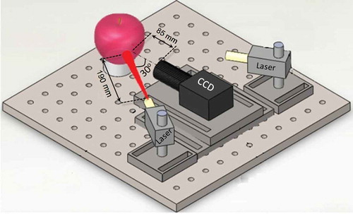
The apples cv. ‘Red Delicious’ (760 samples) were used in this study. The number of 540 apples was kept at 85 ± 5% relative humidity and 0 ± 1°C for five months. To accelerate the mealiness development in samples, the remaining 220 apples were stored under 20°C and relative humidity of 95% as recommended by FAIR standard.^[23] The schematic of biospeckle imaging setup is shown in Figure 1. It consisted of a CCD camera (8-bit depth, Model No: BCP-1050MT, Korea) equipped with a zoom lens (18–120 mm, Avenir CCTV lens, Japan) which located at the distance of 85 mm from the sample. Also there were two 680 and 780 nm laser diodes (3 mW) which impinged on the sample surface at the angle of 30° and the distance of 190 mm (Figure 1). First, the samples were illuminated (covering an area about 78.5 mm²) by the laser emitting at 680 nm, and then, biospeckle images (480 × 720 pixels) were recorded during 25 s (equal to 500 image frames) at a rate of 20 fps. This procedure was followed by exposing the samples to the laser beam of 780 nm.

Figure 1. Schematic of biospeckle imaging setup.

Confined compression test

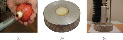
To measure the texture attributes of apples destructively, cylindrical samples were extracted just from the same imaging area (Figure 2(a)). Each sample was 17 mm in height and diameter. The samples were confined in a disc hole made of stainless steel with the same size of the samples (Figure 2(b)). A deformation of 2.5 mm was applied on each sample at the speed of 0.33 mm s⁻¹ by a texture analyser (TA.XTplus, Stable Micro Systems Inc., Surrey, UK) equipped with a probe of 15.3 mm in diameter (Figure 2(c)). On the other hand, the released juice during the compression test was collected by a filter paper located beneath the sample. Two parameters were measured in the compression test. One parameter was juiciness expressed as the juice-soaked area on the paper (expressed in cm²), and the other was stiffness defined as the force-deformation curve slope (expressed in kN m⁻¹). According to the stiffness and juiciness parameters, apple samples were classified into non-mealy and mealy groups. An apple was labelled mealy when its stiffness and juiciness parameters were less than 20 kN m⁻¹ and 5 cm², respectively. Otherwise, it was considered as a non-mealy apple. Furthermore, non-mealy apples were also separated into fresh and semi-mealy groups. A firm (stiffness ≥20 kN m⁻¹) and juicy (juiciness ≥5 cm²) apple was labelled as fresh. Otherwise, it was called a semi-mealy sample. The threshold values for stiffness and juiciness were selected according to Arefi et al.^[22]

Figure 2. The confined compression test procedure; (a) extraction of a cylindrical sample, (b) the sample confined in a stainless steel disc, (c) compression of the sample.

Configuration of time-history speckle pattern (THSP) image

As mentioned above, the number of 500 image frames lasting 25 s was recorded for each sample. The middle column of each frame was extracted and set side by side to make a new image, called time-history speckle pattern (THSP). THSP is one of the mostly used approaches to evaluate the biospeckle activity. In a THSP image, horizontal and vertical directions represent time and spatial information, respectively.^[24] In this study, the height of a THSP image was 400 pixels and its horizontal length was considered 500 (Figure 3(a)), lasting 25 s), 300 (Figure 3(b), lasting 15 s), 100 (Figure 3(c), lasting 5 s), 50 (Figure 3(d), lasting 2.5 s), and 20 (Figure 3(e), lasting 1 s) pixels. In other words, the time required to make a THSP image ranged from 1 to 25 s.

Figure 3. An example of time historical speckle patterns (THSP) at the wavelength of 680 nm: (a), (b), (c), (d), and (e) represent THSP images at the recording times of 25, 15, 10, 5, 2.5, and 1 s, respectively.

Evaluation of THSP images

The common biospeckle features

In this study, the common biospeckle terms refer to those features which has been very common in evaluation of THSP images and already used by other researchers. This group included IM, the absolute values of difference (AVD), and autocorrelation features. A detailed description is given in Arefi et al.^[22]

Image texture features

Texture is an important feature used in the description of an image. Although there is not a clear definition for texture of an image, it relates to both the grey-level intensity and the location of pixels. To date, several approaches have been introduced to describe textural properties of images. Since it is difficult to identify the best kind for a certain application, different approaches are often applied together. In the present study, Statistical and Transform-based texture analysis methods, as the two mostly used approaches in food industry, were used to analyse THSP images.^[25,26] Statistical texture analysis methods included the first order statistics (8 features), grey-level co-occurrence matrix (40 features), grey-level run length matrix (44 features), and local binary pattern (8 features). On the other hand, wavelet (72 features) and Gabor transform (96 features) were used as transform-based approaches. These methods are briefly described in the following subsections.

First order statistics (FOS)

First order statistics are the simplest features in image texture analysis that correspond to brightness value of each pixel, regardless of the relationship between neighbouring pixels. In this method, the number of pixels h(z_i) with grey-level intensity i is counted to make a gray-level histogram. Afterward, the histogram is normalized by Eq. (1)^[26]:

(1)

where h(z_i), p(z_i), and n are the image histogram, the normalized histogram, and the total number of pixels in the image, respectively. In the present study, 8 statistical features were extracted from each THSP normalized histogram as listed in Table 1.

Table 1. Texture features extracted from each THSP image.

Features extracted from the image histogram and local binary pattern		Features extracted from gray-level co-occurrence matrix		Features extracted from gray level run length matrix
Description	Formula^a	Feature name	Formula^b	name	Formula^c
Mean		Maximum of probability		Short run emphasis
Standard deviation		Homogeneity		Long run emphasis
Skewness		Correlation		Gray level non-uniformity
Kurtosis		Dissimilarity		Run length non-uniformity
Smoothness		Variance		Run percentage
Coefficient of variation		Contrast		Low gray level run emphasis
Uniformity		Uniformity		High gray level run emphasis
Entropy		Entropy		Short run low gray level emphasis
		Cluster shade		Short run high gray level emphasis
		Cluster prominence		Long run low gray level emphasis
				Long run high gray level emphasis

^az_i is a random variable indicating intensity, p(z_i) represents the histogram of the intensity levels, L indicates the number of intensity levels and µ shows the mean.

^bσ, µ, and (i, j) represent the mean, standard deviation, and normalized gray level co-occurrence matrix, respectively.

^cRLM is grey level run length matrix, N_g and N_r are number of gray levels and run lengths, and n_p is the sum of image pixels.

Gray-level co-occurrence matrix (GLCM)

A GLCM is a function of distance and orientation between neighbouring pixel pairs in which the number of pixel pairs at distance d and direction θ is counted, and consequently a GLCM is constructed. According to researches done by Zheng et al.^[25] and Mollazade et al.^[26], the values of 0, 45, 90, and 135° were selected for the direction θ, while the distance parameter d was set to one pixel. After making the GLCM, it was normalized by Eq. (2)^[25]:

(2)

where COM(k, l), N_com(k, l), and N represent co-occurrence matrix, normalized co-occurrence matrix, and the sum of elements in co-occurrence matrix, respectively. Each normalized GLCM was then analysed using 10 features suggested by Haralick et al.^[27] (Table 1). A total of 40 features (4 direction × 10 statistical features) were extracted from each THSP image.

Gray-level run length matrix (GLRLM)

GLRLM corresponds to the number of consecutive pixels with similar grey value in a specific direction of an image. The consecutive pixels with the same grey value are called run and the number of pixels in the run is considered as length run. In a GLRLM, each element RLM(i, j) represents the total number of occurrences of the length run j with grey value i, in the direction θ. Four directions θ = 0, 45, 90, and 135° were used in this study to make four separate GLRLM of each THSP image. Afterwards, 11 features, as suggested by Tang^[28], were extracted from each GLRLM (Table 1). Totally, 44 features (4 direction × 11 GLRLM texture descriptors) were extracted from each THSP image.

Local binary pattern (LBP)

To make a LBP, usually a 3 × 3 neighbourhood of pixels is defined. At each location (x, y), a comparison is made between the neighbouring pixels and the central pixel. Each neighbouring pixel gets the value of one if its grey value is greater or equal to that of the central pixel. Otherwise, it is replaced with the value of zero. Then the binary values are multiplied by the weights generated from Eq. (3), and their sum is allocated to the central pixel. This is processed to the whole image in turn.

(3)

where , p_n, p_c, and L are the value of the neighbouring pixel, the value of the central pixel, and the number of neighbouring pixels, respectively. As can be found from Eq. (3), LBP is not rotational invariant and thus different values can be obtained according to indexing of the neighbouring pixels. To make LBP resistant against rotation, each possible number was obtained in the clockwise rotation and the maximum number was selected. In this study, eight statistical features were extracted from the normalized histogram of LBP (Table 1).

Wavelet transform

Fourier and wavelet transforms are two popular frequency analysis techniques. Applying a Fourier transform is suitable when the stationary condition is satisfied by a signal. However, no stationary condition requires in implementation of wavelet transform. Since the stationary condition is unknown in working with the biospeckle phenomenon, it is more suggested to use wavelet instead of Fourier transform.^[29] Discrete wavelet transform for a function f(x, y) is defined by Eq. (4)^[30]:

(4)

where W is discrete wavelet coefficient, ψ is wavelet-mother function, M and N are image size, j is the scale parameter, and m and n are location parameters. In 2-D discrete wavelet transform, the image rows are first passed through the low and high frequency filters. It is followed by passing the columns through the same filters, and thus, four sub-images are resulted in. These sub-images are called Approximation, Horizontal, Vertical, and Diagonal details.^[30] This process can be repeated several times and each iteration is called one decomposition level. In this study, each THSP image was decomposed into three levels using fourth-order Daubechies wavelet (Db4). Each level of decomposition was described using mean, standard deviation, skewness, kurtosis, energy, and entropy. A total of 72 features (6 statistical features × 3 decomposition levels × 4 wavelet coefficients) were extracted from each THSP image.

Gabor transform

Gabor transform, also known as Gabor filter, is a kind of wavelet transform with a specific mother wavelet function (a Gaussian function modulated by a sinusoidal function). Gabor filter generates power responses when it matches the local specific frequencies and directions. Therefore, two parameters, direction (θ) and frequency (f), are needed to be selected before applying the filter. Four frequencies f = 0.17, 0.25, 0.35, and 0.5 Hz at four direction values of 0, 45, 90, and 135°, as suggested by Mollazade et al.^[26], were used in this study. After applying the Gabor transform on THSP images, six statistical features including mean, standard deviation, skewness, kurtosis, energy, and entropy were measured. In total, 96 features (6 statistical features × 4 frequencies × 4 directions) were extracted from each THSP image.

Prediction and discriminant models

ANN models (developed in Matlab software) were applied to predict the stiffness and juiciness. To avoid over-fitting in development of ANN models, the most relevant features were selected using the stepwise discrimination analysis method. Apart from the feature selection, the number of hidden layers and neurons are important in ANN models.^[31] In the current study, ANN models with one hidden layer including different neuron numbers were developed. The 75% of data were used for the calibration (60% for training and 15% for cross-validation) and the evaluation of the models was carried out with the remaining data. The correlation coefficient (r) and the standard error (SE) parameters (Eq. 5 and 6) were used to quantify the performance of the prediction models.^[32] The best models attributed to higher correlation coefficient and lower standard error.

(5)

(6)

where , p_i is the predicted value by model, m_i represents the measured value in the destructive test, represents the mean predicted values, represents the mean measured values, and n is the number of samples. Furthermore, classification of apples according to their mealiness levels was carried out using ANN models developed in the same way as the prediction models were developed. The classification accuracy (Eq. 7) and total classification accuracy (Eq. 8)) were used as performance evaluation criteria of the classification models.

(7)

(8)

where T_p is the number of true positive, F_p is the number of false positive, T_n is the number of true negative, and F_n is the number of false negative.

Results

ANN prediction models for the apple stiffness and juiciness

Common biospeckle features

The results of calibration and validation stages for the prediction of stiffness and juiciness are summarized in Table 2. ANN models developed based on the data acquired during 25 s showed relatively better performances as compared to the others. The stiffness was predicted with r values equal to 0.56 and 0.52, and standard errors of 9.7 and 10.2 kN m⁻¹ at 680 and 780 nm, respectively. The models were able to predict the apple juiciness with r = 0.57 and SEP = 2.6 cm² at 680 nm, and r = 0.58 and SEP = 2.6 cm² at 780 nm. By reducing the recording time, ANN models resulted in worse results for both the stiffness and juiciness. At the recording time of 1 s, the highest prediction r values for the stiffness and juiciness were 0.25 and 0.29, respectively.

Table 2. Prediction of apple stiffness and juiciness by ANN models.

				Calibration		Validation
Feature description	Quality attributes	Laser wavelength (nm)	Image No. (Frame)/Recording time (s)	r	SECV^a	r	SEP^a
Common biospeckle features	Stiffness (kN m^−1)	680	500/25	0.59	9.4	0.56	9.7
			300/15	0.55	9.7	0.53	9.9
			100/5	0.43	10.4	0.41	10.8
			50/2.5	0.35	10.8	0.35	11.2
			20/1	0.32	11.1	0.25	11.3
		780	500/25	0.52	9.9	0.52	10.2
			300/15	0.51	10.2	0.44	10.6
			100/5	0.46	10.4	0.40	10.9
			50/2.5	0.36	10.8	0.35	10.9
			20/1	0.23	11.3	0.21	11.5
	Juiciness (cm^2)	680	500/25	0.59	2.5	0.57	2.6
			300/15	0.58	2.6	0.54	2.7
			100/5	0.48	2.7	0.43	2.9
			50/2.5	0.38	2.8	0.38	2.9
			20/1	0.29	3.0	0.29	3.1
		780	500/25	0.63	2.5	0.58	2.6
			300/15	0.57	2.6	0.55	2.6
			100/5	0.49	2.8	0.43	2.9
			50/2.5	0.33	2.9	0.33	3.0
			20/1	0.26	2.9	0.20	3.1
Texture features	Stiffness (kN m^−1)	680	500/25	0.71	8.2	0.70	8.4
			300/15	0.71	8.3	0.69	8.6
			100/5	0.70	8.1	0.70	8.4
			50/2.5	0.73	8.1	0.69	8.5
			20/1	0.71	8.1	0.71	8.3
		780	500/25	0.61	9.4	0.57	9.7
			300/15	0.62	9.1	0.60	9.3
			100/5	0.62	9.3	0.58	9.6
			50/2.5	0.61	9.4	0.61	9.5
			20/1	0.58	9.4	0.58	9.6
	Juiciness (cm^2)	680	500/25	0.68	2.3	0.68	2.3
			300/15	0.71	2.3	0.68	2.3
			100/5	0.66	2.4	0.64	2.4
			50/2.5	0.67	2.3	0.67	2.3
			20/1	0.68	2.3	0.66	2.4
		780	500/25	0.65	2.4	0.63	2.5
			300/15	0.67	2.4	0.65	2.4
			100/5	0.66	2.4	0.62	2.5
			50/2.5	0.64	2.4	0.62	2.5
			20/1	0.66	2.4	0.64	2.5

Texture features

The best results in the prediction of stiffness and juiciness attributes were obtained for the models developed at 680 nm (Table 2). At the recording time of 25 s, the models resulted in r = 0.70 and SEP = 8.4 kN m⁻¹ for the stiffness. These results showed 25% improvement in r value and about 13% improvement in SEP for the validation stage compared with the models developed by the common biospeckle features. For THSP images consisted of 20 frames (lasting 1 s), the correlation between the predicted and measured stiffness for validation was 0.71 with the SEP = 8.3 kN m⁻¹. In addition, the prediction of juiciness at 680 nm and for the recording time of 25 s resulted in the correlation coefficient and the standard error of 0.68 and 2.3 cm², respectively (Table 2). It showed relatively better performance in comparison with the models developed by the common biospeckle features. When the recording time was reduced to 1 s, the models for the prediction of juiciness resulted in r = 0.66 and SEP = 2.4 cm² which were much better than those of the models developed by the common biospeckle features (r = 0.29 and SEP = 3.1 cm²).

ANN discriminant models for the mealiness classification

Common biospeckle features

ANN classification results of non-mealy and mealy apples are presented in Table 3. At the recording time of 25 s, the model achieved the classification accuracy of 76.8 and 80.6% for non-mealy apples at the wavelengths of 680 and 780 nm, respectively. As seen in Table 3, mealy apples were classified with the accuracy of 77.3% (at 680 nm) and 70.9% (at 780 nm). Much poorer classification accuracy was achieved for mealy apples when it was attempt to reduce the recording time. For the recording time of 1 s, only 46.8 and 55.9% of mealy apples were correctly classified at 680 and 780 nm, respectively. On the other hand, classification accuracies of fresh and semi-mealy samples at 680 nm and the recording time of 25 s were 76.7 and 64.1%, respectively (Table 3). At the wavelength of 780 nm, classification accuracies of 81.7 and 70.9% were, respectively, obtained for fresh and semi-mealy apples. With reducing the recording time to 1 s, a higher misclassification rate was obtained for semi-mealy apples at both wavelengths (Table 3).

Table 3. Classification results of apples according to the mealiness level by ANN models.

			Calibration (%)			Validation (%)
			Classification accuracy			Classification accuracy
Feature description	Laser wavelength (nm)	Image No. (Frame)/Recording time (s)	Non-mealy	Mealy	TCA^a	Non-mealy	Mealy	TCA
Common biospeckle features	680	500/25	77.4	76.1	76.8	76.8	77.3	76.9
		300/15	75.8	83.7	79.1	77.8	64.5	76.2
		100/5	80.2	44.2	65.3	88.5	37.3	82.3
		50/2.5	88.3	18.9	59.5	89.9	20.5	81.5
		20/1	86.5	37.4	66.1	88.0	46.8	83.0
	780	500/25	78.7	81.6	79.9	80.6	70.9	79.4
		300/15	85.4	76.8	81.9	82.8	65.9	80.8
		100/5	90.5	60	77.9	85.7	50.0	81.4
		50/2.5	90.8	51.6	74.5	89.1	47.7	84.1
		20/1	84.0	65.8	76.5	81.9	55.9	78.7
Texture features	680	500/25	86.2	94.7	89.7	86.3	95.5	87.4
		300/15	85.0	94.7	89.0	86.9	94.1	87.8
		100/5	85.2	90.0	87.2	85.2	95.0	86.3
		50/2.5	85.2	89.5	87.0	83.3	97.3	85.0
		20/1	84.5	93.7	88.3	83.8	85.5	84.0
	780	500/25	81.6	83.2	82.3	86.5	74.1	85.0
		300/15	82.9	84.2	83.5	88.0	75.5	86.5
		100/5	87.6	73.2	81.6	87.0	70.5	85.0
		50/2.5	82.8	81.6	82.3	87.7	76.4	86.3
		20/1	87.3	81.6	84.9	88.6	71.4	86.5
			Fresh	Semi-mealy		Fresh	Semi-mealy
Common biospeckle features	680	500/25	72.7	75.2	73.9	76.7	64.1	74.5
		300/15	80.5	72.2	76.6	85.7	50.4	79.6
		100/5	80.2	61.7	71.6	79.9	46.3	74.1
		50/2.5	75.8	29.1	53.9	83.4	23.0	72.9
		20/1	76.7	52.2	65.2	82.8	50.7	77.2
	780	500/25	83.6	72.4	78.3	81.7	70.9	79.8
		300/15	78.6	60.9	70.3	76.3	69.3	75.1
		100/5	79.6	57.8	69.4	81.5	59.6	77.7
		50/2.5	81.6	36.1	60.2	86.7	38.9	75.5
		20/1	78.5	35.2	58.2	83.6	23.7	73.2
Texture features	680	500/25	85.7	63.5	75.3	86.3	65.9	82.8
		300/15	86.5	72.6	80.0	86.0	66.3	82.6
		100/5	87.5	71.7	80.1	89.4	70.7	86.2
		50/2.5	87.2	68.3	78.3	85.3	65.6	81.9
		20/1	86.9	62.6	75.5	88.2	68.5	84.8
	780	500/25	78.8	66.1	72.9	83.7	62.6	80.1
		300/15	81.0	65.7	73.8	83.2	55.2	78.3
		100/5	85.6	56.5	72.0	79.5	47.8	74.0
		50/2.5	82.4	62.6	73.1	79.3	48.1	73.9
		20/1	83.2	58.7	71.7	83.0	57.0	78.5

^aTCA = Total classification accuracy.

Texture features

Texture-ANN models resulted in high classification accuracy for mealy and non-mealy apples (Table 3). For the recording time equal of 25 s, the models developed at 680 nm achieved 86.3 and 95.5% classification accuracy for non-mealy and mealy samples, respectively. Also at 780 nm, non-mealy and mealy apples were classified with the accuracies of 86.5 and 74.1%, respectively. Even though the recording time was reduced to 1 s, ANN models were still successful in classification of non-mealy (83.8% at 680 nm and 88.6% at 780 nm) and mealy apples (85.5% at 680 nm and 71.4% at 780 nm). Moreover, at the wavelength of 680 nm, the highest classification accuracies of fresh (89.4%) and semi-mealy (70.7%) apples belonged to the recording time of 15 s. By reducing the recording time to 1 s, classification accuracies of 88.2% and 68.5% were obtained for fresh and semi-mealy apples, respectively (Table 3). At the wavelength of 780 nm and the recording time of 25 s, fresh and semi-mealy apples were classified with the accuracies of 83.7 and 62.6%, respectively; reducing the recording time to 1 s resulted in classification accuracies of 83% (for fresh) and 57% (for semi-mealy), (Table 3).

Discussion

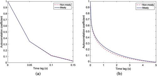
According to the results, the shorter recording times caused higher misclassification rate for mealy apples when the common biospeckle features were used as inputs in the model development. However, the classification accuracy of non-mealy groups was increased from 76.8% to 89.9% at 680 nm, and from 80.6% to 89.1% at 780 nm when the recording time was reduced from 25 to 2.5 s. This may be because of the biospeckle activity of non-mealy and mealy groups. For the short recording times (e.g. 1 s), biospeckle activity of mealy apples was similar to that of non-mealy ones (Figure 4(a)). It thus resulted in misclassification of mealy apples as non-mealy samples, because the number of non-mealy apples was higher and the calibration models tended to detect them much more. On the other hand, the difference in biospeckle activity between mealy and non-mealy groups became more when the recording time was long enough (e.g. 25 s), and thus, it resulted in better classification accuracies (Figure 4(b)). Similar behaviour was found for fresh and semi-mealy samples as the difference in biospeckle activity increased by increasing the recording time. As a result, the correct classification rate increased for fresh groups when the recording time decreased, while semi-mealy apples were detected with poorer accuracies because they were labelled as fresh ones. Apart from the classification models, poor results were obtained for prediction of apple texture attributes (stiffness and juiciness) when the recording time was reduced to 1 s. It can be concluded that the common biospeckle features are completely depended on the recording time and good results can be obtained only when the recoding time is long enough. In comparison with the biospeckle features-based models, both prediction and discriminant models showed better performance when the image texture features were used as inputs in the model development. The texture features-based models were relatively independent of the recording time. The models corresponding to short recording times performed as perfect as those developed at 25 s. Regardless of the kind of image descriptors, the calibration models provided poor results for the prediction of apple stiffness (r ≤ 0.71 and SEP≥ 8.3 kN m⁻¹) and juiciness (r ≤ 0.68 and SEP≥ 2.3 cm²). Difficulty in accurate prediction of apple stiffness (r ≤ 0.76 and SEP≥ 10.6 kN m⁻¹) and juiciness (r ≤ 0.54 and SEP≥ 1.29 cm²) has been already reported by Huang and Lu (2010) when hyperspectral scattering imaging was used. In comparison with the prediction models, better results were achieved for classification of apples. Fresh (≤89% accuracy) and mealy (≤95% accuracy) apples were classified with acceptable accuracies, even though misclassification rate (>30%) was high for semi-mealy apples. This can be due to the fact that fresh and mealy apples are such different in texture attributes (stiffness and juiciness) and consequently biospeckle behaviour makes them easy to separate. In summary, further investigation is suggested to achieve the better performance regarding both prediction and classification models.

Figure 4. Biospeckle activity of non-mealy and mealy apples measured by autocorrelation function for the recording times of 1 s (a) and 25 s (b).

Conclusion

Analysing biospeckle images using the texture descriptors in comparison with the common biospeckle ones showed that it would be possible to achieve higher apple mealiness classification accuracies at short recording times. Even though further work is still needed to reach a comprehensive conclusion on this, the findings of the current study can be considered as an introduction towards making biospeckle imaging a faster technique through replacing the common biospeckle descriptors by the texture-based ones, and therefore, removing barriers in the way of its online application.

References

- Barreiro, P.; Ortiz, C.; Ruiz‐Altisent, M.; Schotte, S.; Andani, Z.; Wakeling, I.; Beyt, P. K. Comparison between Sensory and Instrumental Measurements for Mealiness Assessment in Apples. A Collaborative Test. J. Texture Stud. 1998, 29, 509–525.
- Harker, F. R.; Hallett, I. C. Physiological Changes Associated with Development of Mealiness of Apple Fruit during Cool Storage. HortScience. 1992, 27, 1291–1294.
- Moshou, D.; Wahlen, S.; Strasser, R.; Schenk, A.; Ramon, H. Apple Mealiness Detection Using Fluorescence and Self-Organising Maps. Comput. Electron. Agric. 2003, 40, 103–114.
- Huang, M.; Lu, R. Apple Mealiness Detection Using Hyperspectral Scattering Technique. Postharvest Biol. Technol. 2010, 58, 168–175.
- Bechar, A.; Mizrach, A.; Barreiro, P.; Landahl, S. Determination of Mealiness in Apples Using Ultrasonic Measurements. Biosystems Eng. 2005, 91, 329–334.
- Barreiro, P.; Moya, A.; Correa, E.; Ruiz-Altisent, M.; Fernandez-Valle, M.; Peirs, A.; Wright, K. M.; Hills, B. P. Prospects for the Rapid Detection of Mealiness in Apples by Nondestructive NMR Relaxometry. Appl. Magn. Reson. 2002, 22, 387–400.
- Barreiro, P.; Ortiz, C.; Ruiz-Altisent, M.; Ruiz-Cabello, J.; Fernández-Valle, M. E.; Recasens, I.; Asensio, M. Mealiness Assessment in Apples and Peaches Using MRI Techniques. Magn. Reson. Imaging. 2000, 18, 1175–1181.
- Mehinagic, E.; Royer, G.; Symoneaux, R.; Bertrand, D.; Jourjon, F. Prediction of the Sensory Quality of Apples by Physical Measurements. Postharvest Biol. Technol. 2004, 34, 257–269.
- Moshou, D.; Wahlen, S.; Strasser, R.; Schenk, A.; De Baerdemaeker, J.; Ramon, H. Chlorophyll Fluorescence as a Tool for Online Quality Sorting of Apples. Biosystems Eng. 2005, 91, 163–172.
- Huang, M.; Zhu, Q.; Wang, B.; Lu, R. Analysis of Hyperspectral Scattering Images Using Locally Linear Embedding Algorithm for Apple Mealiness Classification. Comput. Electron. Agric. 2012, 89, 175–181.
- Mollazade, K.; Arefi, A. Optical Analysis Using Monochromatic Imaging-Based Spatially-Resolved Technique Capable of Detecting Mealiness in Apple Fruit. Sci. Hortic. 2017, 225, 589–598.
- Arefi, A.; Ahmadi Moghaddam, P.; Mollazade, K.; Hassanpour, A.; Valero, C.; Gowen, A. Mealiness Detection in Agricultural Crops: Destructive and Nondestructive Tests: A Review. Compr. Rev. Food Sci. Food Saf. 2015, 14, 657–680.
- Zdunek, A.; Adamiak, A.; Pieczywek, P. M.; Kurenda, A. The Biospeckle Method for the Investigation of Agricultural Crops: A Review. Opt. Lasers Eng. 2014, 52, 276–285.
- Braga, R. A.; Dupuy, L.; Pasqual, M.; Cardoso, R. R. Live Biospeckle Laser Imaging of Root Tissues. Eur. Biophys. J. 2009, 38, 679–686.
- Adamiak, A.; Zdunek, A.; Kurenda, A.; Rutkowski, K. Application of the Biospeckle Method for Monitoring Bull’s Eye Rot Development and Quality Changes of Apples Subjected to Various Storage methods—Preliminary Studies. Sensors. 2012, 12, 3215–3227.
- Pajuelo, M.; Baldwin, G.; Rabal, H.; Cap, N.; Arizaga, R.; Trivi, M. Bio-Speckle Assessment of Bruising in Fruits. Opt. Lasers Eng. 2003, 40, 13–24.
- Amaral, I. C.; Braga, R. A., Jr; Ramos, E. M.; Ramos, A. L. S.; Roxael, E. A. R. Application of Biospeckle Laser Technique for Determining Biological Phenomena Related to Beef Aging. J. Food Eng. 2013, 119, 135–139.
- Zdunek, A.; Herppich, W. B. Relation of Biospeckle Activity with Chlorophyll Content in Apples. Postharvest Biol. Technol. 2012, 64, 58–63.
- Zdunek, A.; Cybulska, J. Relation of Biospeckle Activity with Quality Attributes of Apples. Sensors. 2011, 11, 6317–6327.
- Rabelo, G. F.; Braga Júnior, R. A.; Fabbro, I. Laser Speckle Techniques in Quality Evaluation of Orange Fruits. Rev. Bras. Eng. Agríc. Ambient. 2005, 9, 570–575.
- Szymanska-Chargot, M.; Adamiak, A.; Zdunek, A. Pre-Harvest Monitoring of Apple Fruits Development with the Use of Biospeckle Method. Sci. Hortic. 2012, 145, 23–28.
- Arefi, A.; Ahmadi Moghaddam, P.; Hassanpour, A.; Mollazade, K.; Modarres Motlagh, A. Non-Destructive Identification of Mealy Apples Using Biospeckle Imaging. Postharvest Biol. Technol. 2016, 112, 266–276.
- FAIR. Mealiness in Fruits. Consumer Perception and Means for Detection. Contract No. FAIR-CT95-0302, 4th Framework Program, European Commission, Directorate-General XII. B-1049, Brussels, 1998.
- Junior, R. A. B.; Silva, B. O.; Rabelo, G.; Costa, R. M.; Enes, A. M.; Cap, N.; Rabal, H.; Arizaga, R.; Trivi, M.; Horgan, G. Reliability of Biospeckle Image Analysis. Opt. Lasers Eng. 2007, 45, 390–395.
- Zheng, C.; Sun, D.; Zheng, L. Recent Applications of Image Texture for Evaluation of Food Qualities—A Review. Trends Food Sci. Technol. 2006, 17, 113–128.
- Mollazade, K.; Omid, M.; Akhlaghian Tab, F.; Rezaei Kalaj, Y.; Mohtasebi, S.; Zude, M. Analysis of Texture-Based Features for Predicting Mechanical Properties of Horticultural Products by Laser Light Backscattering Imaging. Comput. Electron. Agric. 2013, 98, 34–45.
- Haralick, R. M.; Shanmugam, K.; Dinstein, I. Textural Features for Image Classification. IEEE Trans. Syst. Man. Cybern. 1973, 6, 610–621.
- Tang, X.;. Texture Information in Run-Length Matrices. IEEE Trans. Image Process. 1998, 7, 1602–1609.
- Nobre, C. M. B.; Braga, R. A., Jr; Costa, A. G.; Cardoso, R. R.; da Silva, W. S.; Sáfadi, T. Biospeckle Laser Spectral Analysis under Inertia Moment, Entropy and Cross-Spectrum Methods. Opt. Commun. 2009, 282, 2236–2242.
- Gonzalez, R. C.; Woods, R. E. Digital Image Processing, second ed.; Prentice Hall: New Jersey, USA, 2002; pp 349.
- Lu, R.;. Nondestructive Measurement of Firmness and Soluble Solids Content for Apple Fruit Using Hyperspectral Scattering Images. Sens. Instrum. Food Qual. Saf. 2007, 1, 19–27.
- Romano, G.; Nagle, M.; Argyropoulos, D.; Müller, J. Laser Light Backscattering to Monitor Moisture Content, Soluble Solid Content and Hardness of Apple Tissue during Drying. J. Food Eng. 2011, 104, 657–662.