Airborne LiDAR point cloud in mapping of fluvial forms: a case study of a Hungarian floodplain

Abstract

The aim of this paper was to analyze the ground and low vegetation points of a Light Detection and Ranging (LiDAR) point cloud from the aspect of the generated digital terrain model (DTM). We determined the height difference between the surveyed surface and the DTM and the level of interspersion of ground and low vegetation points in a floodplain. Finally, we performed a supervised classification with topographic (elevation, slope and aspect) variables and an Normalized Difference Vegetation Index (NDVI) layer to identify swales and point bars as floodplain forms. Cross sections of field surveys provided reference data to express the magnitude of the bias on the DTM caused by the vegetation, and we proved that the bias can reach the 60% of the relative height and depth of the floodplain forms (mean error was 0.15 ± 0.12 m). A landscape metric, the Aggregation Index, provided an appropriate tool to analyze and quantify the interspersion of the ground and vegetation points: indicating a high level of interspersion of the classified points, i.e. proved that vegetation points where the last echoes reflected from the vegetation became ground points. Floodplain classification performed best with the common use of DTM, slope, aspect and NDVI coverages, with 71% overall accuracy.

Keywords:

• geomorphology
• fluvial landform
• point cloud
• landscape indices
• Aggregation Index

1. Introduction

Floodplains play an important role in countries with low relief such as Hungary. They represent an outstanding value as natural resources, i.e. they provide cultivable soils, groundwater resources and valuable habitats and also function as important ecological corridors (Balogh, Kiss, and Fiala 2016; Dollar et al. 2007; Lóczy, Pirkhoffer, and Gyenizse 2012; Nyarko et al. 2015; Ortmann-Ajkai et al. 2014; Schindler et al. 2016). Flood among natural processes, including socioeconomic drivers, plays a dominant role in shaping surface form and structure. Therefore, an accurate information of surface form and structure is crucial in management of floodplain agricultural, floodplain nature conservation and surface water retention (Kiss and Sándor 2009; Kundrát et al. 2016; O’ Connell et al. 2007; Surian 1999; Tälle et al. 2016; Tarolli and Sofia 2016; Timár and Gábris 2006).

Floodplain surfaces are spatially complex geomorphic landscapes with a high diversity of surface features and landforms (Szabó, Vass, and Tóth 2012; Thoms 2003). From a geomorphic perspective, a floodplain can be considered a macroform (Lóczy, Pirkhoffer, and Gyenizse 2012) which is characterized by the typical assemblage of its mesoforms (point bars, levees, oxbows, backswamps, swales etc.) and even the microforms (ripples, dunes) superimposed on them (Lewin 1978). This spatial complexity influences regional hydrodynamics, ecological productivity and agricultural practices and causes accumulation of heavy metals (Ciszewski 2003; Hughes 1997; Middelkoop 2000; Nguyen et al. 2009; Szalai 1998; Tamás and Farsang 2011). Thus, accurate morphological characteristics data will be useful for flood mitigation purposes as well (Sofia, Dalla Fontana, and Tarolli 2014).

Field surveys or topographic maps do not provide enough resolution to obtain detailed characteristics of the micro-topography of the floodplain (Balogh, Kiss, and Fiala 2016). A simple visual inspection of fine elevation data can often go beyond the detail that is available in hand-drawn classical geomorphological maps (Seijmonsbergen, Hengl, and Anders 2011). Classic geomorphological mapping is also thought to be subjective, nonreproducible and time consuming (Verstappen 2011); as a result, traditional geomorphological maps are slowly being replaced by geomorphological maps which are extracted from digital terrain models (DTMs) (Drǎguţ et al. 2013).

Among the remote-sensing technologies currently available, Light Detection and Ranging (LiDAR) provides the highest resolution topographic data with noticeable advantages over traditional surveying techniques (Tarolli 2014). This technology assists in capturing the surface character and variability and affords accurate spatial information in a 3D environment (Scown, Thoms, and Jager 2015; Szabó et al. 2016). It helps to quantify the spatial characteristics of floodplain features and offers the possibility of an objective, robust and reproducible analysis of the landforms (Passalacqua, Hillier, and Tarolli 2014). The potential of the technology can be useful in mapping and identifying the structure of the vegetation, the land cover and the surface of landforms (Alexander et al. 2015; Ghuffar et al. 2013; Király, Brolly, and Burai 2012; Singh et al. 2012; Zlinszky et al. 2015). However, the topographic LiDAR system has its limitations: the footprint of the laser beam has a diameter of 0.2–0.3 m; consequently, horizontal accuracy cannot be better than the footprint itself. Furthermore, the laser beam is absorbed by the water; a smaller portion of a laser beam reaches to the ground in areas of a sense vegetation, and so, less information is available from the surface. These issues affect the accuracy of the resultant DTM and digital surface model (DeWitt, Warner, and Conley 2015; Podhoranyi and Fedorcak 2015; Riaño et al. 2007).

In previous studies, we can find examples of the application of LiDAR data in fluvial geomorphology and flood risk assessment (Balogh, Kiss, and Fiala 2016; Deshpande 2013; Jones et al. 2007; Notebaert et al. 2009; Ramos, Maruffo, and González 2009; Rapinel, Hubert-Moy, and Clément 2011), but there is hardly research work that focuses on detection of fluvial forms. The question is whether we can identify paleo-channels, swales, point bars, oxbow lakes, cutoff meanders and riverbeds using a DTM derived from an airborne laser scanning campaign.

The aim of this paper is to reveal the possibilities of using LiDAR data in the identification of floodplain elements. We also sought to quantify the bias on DTMs caused by vegetation and to develop an approach to quantify the interspersion of the ground and low vegetation points of the point cloud. The main goal was to perform a supervised classification on the topographic elevation (elevation, slope and aspect) and the Normalized Difference Vegetation Index (NDVI) layers for feature extraction. Our work devotes special attention to swales and point bars among floodplain landforms.

2. Material and methods

2.1. Study area

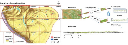
The Tisza River is the longest tributary (977 km) of the Danube River with a catchment of 157,180 km², which is shared by five countries, Ukraine, Romania, Slovakia, Hungary and Serbia (Nguyen et al. 2009). The Tisza River becomes a typical plain-tract river below the town of Tokaj, NE-Hungary (Hamar and Sárkány-Kiss 1999), where our study area is located (Figure 1). The floodplain in the study area is wide, in some cases wider than 4 km. Floodplain development is not restricted by anthropogenic built elements within the levee; thus, the different geomorphological landforms can still be found: swales, point bars, paleo river channels and backswamps. All of these forms developed as the consequence of the lateral accretion of the former Tisza riverbed, i.e. because of changing discharge (biased by the climate) the central line drifted horizontally, and formed its environment. It eroded a new riverbed and, on the opposite side, deposits accumulated to establish the floodplain elements (Schweitzer, Nagy, and Alföldi 2002). According to our field surveys and visual interpretation, there were two levees with a convex shape, and there was one paleo river channel and two backswamps with a concave cross section, which usually contained some water, in varying quantity. The main surface elements of the area were point bars (105 in total), and swales (124; Figure 2), which formed a series of convex and concave landscape elements (Figure 3). The height differences between them are at most a couple of (1–2) meters, but they have a significant effect on the water conditions and also on the vegetation cover. Both forms were covered by grass, bushes and trees, but swales had denser vegetation and they also had water cover (10 out of 124). Due to flooding, the evolution of landforms is continuous. The most intensive floods occur regularly due to snow-melt, which rarely reaches record heights but is rather a sequence of several smaller flood waves, and the intensive precipitation caused by heavy spring rainfall, which is particularly noteworthy if it joins the riverbed already filled by winter floods. Floods do not occur every year and depend on the winter precipitation and the distribution and amount of rainfall in the spring and early summer periods (Hamar and Sárkány-Kiss 1999; Timár and Gábris 2006; Vári, Linnerooth-Bayer, and Ferencz 2003).

Figure 1. Location of the study area. For full colour versions of the figures in this paper, please see the online version.

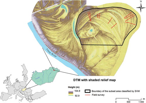
Figure 2. Sampling of the point cloud to analyze the interspersion of the classified points.

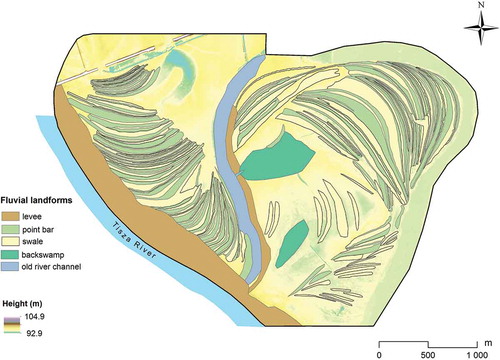
Figure 3. The visually interpreted fluvial landforms.

There is extensive farming activity in this part of the floodplain. The current land uses are grazing and harvesting of hay, forestry with plantations of hybrid poplar and agriculture (mainly fast-growing crops which appear only on the western, and south-western part of the study area with a minimal extent). The types of habitats and vegetation are closely related to typical riparian lands. Soft-wood riparian forest is common on the study site with willow and poplar species, but because of the regulation of the river course, the size and distribution of these habitats have decreased, according to Hamar and Sárkány-Kiss’s (1999) study. As wetland vegetation is severely influenced by ground water (Bölöni et al. 2008), it is more frequent in the lower parts of the terrain, where it makes up 8% of the surface area; woodland and shrubs cover approximately 16% of the study area, and the majority of the remaining area is grassland.

2.2. Dataset

Aerial and LiDAR surveys of the study area were carried out by a Cessna C-206 Skywagon aircraft with a Riegl LMS-Q680i laser scanner and a DigiCam H39 camera, at a flight altitude of 688 m on 20 August 2012. The LiDAR point density was 4 point/m² and the vertical and horizontal accuracy was ±15 cm. A hyperspectral survey was also conducted with an AISA Eagle II sensor on the same day at a height of ~1500 m, in a 400–1000-nm range (5 nm bandwidth, 1285 bands, geometrical resolution was 1.5 m). Both surveys were funded by the Swiss-Hungarian Programme (SH/2/6 project). In accordance with our objectives, we applied the point cloud in the analysis (Figure 4) but also included the hyperspectral image as auxiliary data: we calculated the NDVI (Rouse et al. 1973), using the 670 and 800 nm bands as red and near-infrared bands (Haboudane et al. 2004). Although NDVI was developed to assess the biomass, it also can help to identify water cover (Szabó, Gácsi, and Balázs 2016). Aerial photos were orthocorrected and this was used also as auxiliary data in the investigation.

Figure 4. The main steps of our workflow.

2.3. Data processing and DTM generation

Point cloud preprocessing was performed by the Envirosense Ltd. Our base dataset was the preprocessed (i.e. classified) point cloud with the following categories: ground; low, medium and high vegetation; nonclassified and noise (Table 2). We excluded outlier data points (i.e. those exceeded a height or slope difference relative to their natural neighbors) in the first stage of DTM generation by considering that floodplains do not experience sudden changes on the terrain. Then, in a 3D environment, we also inspected the data visually for anomalies to remove voids, data errors, outlying points and obvious misclassifications. Interpolation was conducted by the Natural Neighbour method at a resolution of 1 m. All analyses were performed using ESRI ArcGIS 10.3 software (ESRI 2014).

Table 1. The average number of points in the cross-section cuboids by floodplain forms (mean ± standard deviation; n: varying width to ensure 30 points/n point density).

Width of cross-section cuboids (m)	Swales	Point bars
4	20.8 ± 12.1	20.9 ± 8.7
6	31.4 ± 18.2	31.3 ± 12.2
8	41.6 ± 23.8	41.2 ± 16.1
10	52.2 ± 30.4	51.1 ± 20.4
n	30	30

Table 2. Characteristics of the point cloud in the study area and by landforms.

	Study area		Point bars		Swales
	Number of points	Points/m^2	Number of points	Points/m^2	Number of points	Points/m^2
Points	93,839,032	9.94	16,179,966	9.82	16,705,014	9.51
Ground points	46,901,456	4.96	9,676,940	5.88	8,629,469	4.91
Missing ground points in a m^2 (%)		11.5		6.8		10.2
Low vegetation points (0–0.5 m)	14,232,174	1.50	2787,820	1.69	3407,885	1.94
Medium vegetation points (0.51–1.50 m)	12,072,124	1.28	1121,205	0.68	2046,105	1.16
High vegetation points (1.51 m)	20,618,516	2.18	2591,643	1.57	2617,142	1.49
Noise	7018	0.00	943	0.00	2111	0.00
Nonclassified	7744	0.00	1415	0.00	2302	0.00

Water surfaces within swales were identified with a field survey and also with a rule-based classification. NDVI has negative values for water bodies (Szabó, Gácsi, and Balázs 2016), and so, we classified NDVI < −0.3 as water and NDVI > −0.3 as non-water classes.

2.4. Analysis of the interspersion of ground and low vegetation points

We randomly designated 25 point bars and 25 swales by visual interpretation and assigned 4, 6, 8, and 10 m wide cross sections (this approach ensured a fixed width per landscape form with a varying number of points per meter for the cross sections). We also carried out a sampling with 30 points/(n)m to ensure the possibility of an investigation with a fixed point number per specific distance (this ensured a fixed number of points with a varying width of sections per landscape form). Following this, we copied these points from the 3D point cloud to new files (altogether there were 125–125 separate files per swale and point bar) and turned them into a vertical 2D projection using their X coordinates as the horizontal axis and the Z coordinates as the vertical axis, with vegetation and ground points representing the attribute data (i.e. class). This approach allowed us to visualize the classified points in a rectangular cuboid, where the width was 4–6–8–10 m or ranged along 30 points/(n)m, the length was the line of the profile and the height was the vertical range of ground and low vegetation points (Figure 5).

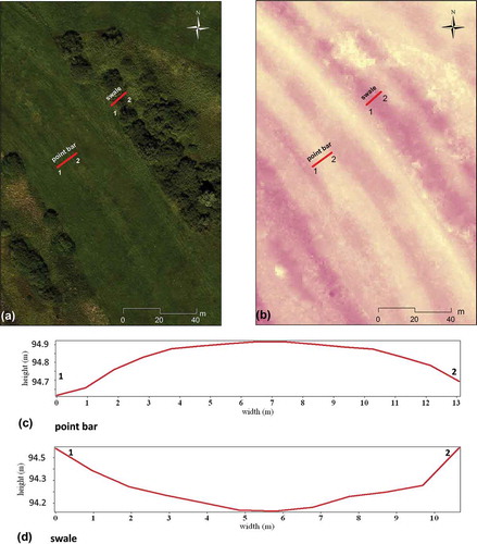
Figure 5. The shape of a characteristic point bar and swale [(a) orthophoto, (b) DTM, (c) profile of the point bar, and (d) profile of the swale).

The interspersion of ground and vegetation points in the cross sections was determined with the contagion (CONTAG) and aggregation (AI) indices in Fragstats 4.2 (Equations (1) and (2)), according to McGarigal and Marks (1995):

(1) $\text{CONTAG}=\frac{2\ln (N)+{\displaystyle {\sum }_{i=1}^N{\displaystyle {\sum }_{j=1}^N\left(\left(n_{ij}/M\right)\ln \left(n_{ij}/M\right)\right)}}}{2\ln (N)}$(1)

where n_ij: i and j were the number of like adjacencies between classes based on the double count method, M was the number of like adjacencies based on the double count method and N the number of classes.

(2) $AI=\left[\frac{g_{ii}}{max-g_{ii}}\right]x100$(2)

where g_ii is the number of like adjacencies between pixels of class i based on the single count method, and max − g_ii is the maximum number of like adjacencies between classes based on the single count method.

As a prerequisite for the calculation, we needed a raster type input; so, we converted 125–125 vector files from both forms to 0.05-m geometric resolution rasters. About 0.05 m may seem excessive, but in the cross-section cuboids, considering the number of points in both vertical (multiple returns) and horizontal perspectives, this was appropriate (Table 1). Our aim was to ensure the adjacency of the pixels, which is the prerequisite of an interspersion analysis. Both CONTAG and AI are ways of quantifying pixel interspersion. Pixels (individually or even in aggregated clusters) in the cross section are handled as patches of a landscape classified into two classes (ground and vegetation); thus, CONTAG and AI can reveal their spatial interspersion. Both indices range from 0% to 100%: 0 represents the maximal disaggregation (without neighboring pixels from the same class) and 100 the maximum aggregation (where the whole area is a single patch). Although the indices do not correlate, they provide the same information on the aggregation of the data points.

AI and CONTAG results were analyzed with null hypothesis testing. The first question was whether the surface height had a significant effect on the interspersion when we sampled the swales and point bars along the profiles with the varying widths. It was important to have enough points to perform the mixture analysis and also to exclude the effect of the topography, i.e. not to measure the interspersion deriving from the changes of the surface height within the sampled profile. Next, we compared the landscape forms based on the AI values.

2.5. Determination of the errors of the DTM

We carried out a field survey with a Stonex S9 RTK GPS, using the “stop-and-go” method with a real-time differential correction of the GNSS permanent station system of Geotrade Ltd (Hungary); vertical and horizontal accuracy was ±1 cm. We surveyed 10 profiles with a length of 230–420 m (Figure 1), crossing 8–15 swale-point bar series. We extracted the elevation data along the profiles of the field survey from the DTM and plotted both data as cross sections in the GIS environment: the X axis was the X coordinate and the Y axis was the elevation. We determined the relative heights and depths of the floodplain forms and also set the differences between the two surface lines at 0.2 m and applied a two-way factorial ANOVA to reveal the effect of the fluvial forms (point bars and swales) and the vegetation, using classes based on their bias on the DTM: clear areas covered by short grass (CL), short grass with hay stocks (HS), areas with reed and tussock forming sedge (R), the same type with dense distribution of tussocks (DR) and woody areas (W).

2.6. Landform classification

DTM and its derivations (slope and aspect) and the NDVI layer were included in the analysis on their own and in several combinations. We applied the Support Vector Machine (SVM) classifier with a radial basis kernel, due to its robustness (Xu, Caramanis, and Mannor 2009) and its effectiveness in classifying data from different sources and dimensions (Bretar et al. 2009). Only swales and point bars were included in the classification – other floodplain forms were limited in number – and they were identified on the basis of the visual interpretation of the orthophoto and the DTM, and a field survey. Random point sampling was applied; then, we divided it into a train and a test sets in a ratio of 70–30% (3500–1500 pixels), respectively. An SVM classification was performed on a subset of the study area, where the swale and point bar topography was one of the most conspicuous (Figure 1). The classification was performed in R 3.3.1 (R Core Team 2016) with the Rattle package 4.1 (Williams 2011). The data preparation and the visualization were conducted in Idrisi Selva (Clark Labs 2012). We reported the overall accuracy (OA) and the producer’s accuracy according to Congalton (1991).

2.7. Statistical analysis

We applied null hypothesis testing to determine the differences among the variables. Normal distribution was controlled with the Shapiro–Wilk test, and accordingly, we applied the t-test for the geomorphometric variables (DTM, aspect and slope) and NDVI (these variables followed the normal distribution), and the Kruskal–Wallis test in the analysis of the interspersion. The Mann–Whitney test was used to reveal whether there is significant difference between the interspersion of swales and point bars, and also as a post hoc test with Bonferroni correction to identify the significant differences between the cross sections with varied widths. Furthermore, we applied the Jonckheere–Terpstra test to reveal if there was a trend along the increasing width of the cross sections. Besides the significance, we also determined the effect sizes (r) which showed the magnitude between the groups in a standardized way, similarly to the correlation coefficient (Cohen 1992; Field 2009). Analyses were performed with R 3.3.1 (R Core Team 2016) using the coin package (Hothorn et al. 2006).

3. Results

3.1. Characteristics of floodplain forms as reflected in the point cloud

Analysis of the point cloud revealed that as a result of the overlapping tracks, the average point density was better than the official 4 points/m², reaching 4.96 points/m² on average, considering the ground points (Table 2). Furthermore, the number of high and low vegetation points (such as trees and grasslands) was the greatest. The proportions of unclassified points and noise were negligible. We removed only 22 ground points as outliers from the floodplain area, confirming the result of the point cloud classification.

Swales and point bars were easy to distinguish visually, based on their appearance (e.g. vegetation, water cover, relative location and relief). The quantified numbers of their characteristics were similar, but due to the aquatic vegetation (e.g. duckweed, tangle and reed) and the higher soil moisture of swales, the vegetation on them was denser, as was reflected in the higher density of vegetation points; additionally, as water absorbs and dense vegetation does not penetrate laser beams, the point density of ground points was slightly lower and the missing ground point ratio was larger for swales than point bars (Table 2). Point bars were slightly higher than swales, and the difference was significant based on the t-test, but its effect size (r) indicated a low magnitude (Table 3). Aspect, slope and NDVI values, however, did not differ, in spite of the visual differences.

Table 3. Comparison of swales and point bars by the applied landscape variables (mean ± standard deviation).

Landscape variable	Point bar	Swale	Mean difference	Sig.	Effect size (r)
DTM (m, a.s.l.)	94.7 ± 0.2	94.5 ± 0.2	0.15	0.003	0.36
Aspect (degree, azimuth)	167 ± 87	174 ± 90	5.80	0.334	0.09
Slope (percent)	0.05 ± 0.03	0.05 ± 0.03	0.002	0.440	0.12
NDVI	0.34 ± 0.09	0.34 ± 0.09	0.008	0.641	0.05

We determined the ground point density of swales and found that in areas of NDVI < −0.3, it was lower (2.68 points/m²), while for NDVI > −0.3, it was denser (3.77 points/m²). This indicated the presence of a water surface, which absorbs laser beams.

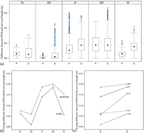
According to the profiles based on the field survey, the relative height of point bars was 0.25 ± 0.10 m and the relative depth of swales was 0.24 ± 0.12 m. We determined that the average error (i.e. the difference between the DTM and the surveyed height) was 0.15 ± 0.12 m (with a maximum of 0.67 m), which was about the 60% of the relative floodplain form heights. On average, the elevation errors of point bars and swales were similar (0.12 and 0.13 m), but considering the vegetation, we found significant differences (Figure 6a). The factorial ANOVA model identified statistically significant (p < 0.001) effects both for fluvial forms and vegetation types, and also for their interaction (Figure 6b and c). The effect of the vegetation type was η_partial = 0.21; the effect of floodplain forms was weak (η_partial = 0.03); their interaction was also weak (η_partial = 0.02) and was only caused by the intersection of woody and clear areas (Figure 6c).

Figure 6. Height differences between the DTM and field survey by floodplain forms and vegetation types (a), and their interaction plot by floodplain forms (b), and by vegetation types (c) (legend: P: point bar; S: swale; CL: clear areas with short grass, R: reed and sedge, DR: dense reed and sedge; W: woods, HS: short (mowed) grass with haystocks).

3.2. Interspersion of the ground and vegetation points of the classified point cloud

The interspersion analysis revealed that AI (Figure 7a) was more sensitive to the wider sampling distance than CONTAG (Figure 7b). It showed significant differences between the different distances according to the Kruskal–Wallis test (χ² = 6.755; p < 0.009), and also a positive trend with the increasing sampling distance based on the Jonckheere–Terpstra test (J–T statistic = 873; p = 0.009). Accordingly, as we needed a sensitive measure, we applied only the AI values to determine the interspersion of the ground and vegetation points. Results showed that the pattern of the points was randomly disaggregated and mixed in all cases, but only the lowest value can be accepted regarding the narrowest sampling distance (4 m), or the value based on a fixed number of points (30 points/(n)m). The mixture of the classified point cloud was similar for swales and point bars in terms of their AI values (mean difference = 0.17; p = 0.937) (Figure 7c).

Figure 7. Interspersion of ground and vegetation points according to AI (a) and CONTAG (b) indices and the mixture of the classified point clouds of swales and point bars (c).

3.3. Landform classification

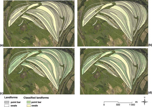
The maps of the floodplain forms resulting from the raster-based SVM classification had an OA range of 55–71% (Table 4). According to the error matrix (Table 4), the most favorable solution was when we took all variables into account; the average error was 26% for point bars and 30% for swales. Using the DTM alone resulted in the most accurate classification for point bars (Figure 8c). Classification of NDVI (Figure 8a), slope (Figure 8b) and aspect performed best for swales; however, this solution was only preferable for the given geomorphic element; the accuracy of the other element was weak (in other words, pixels were classified almost homogeneously to one class, which was not acceptable).

Table 4. Error matrix of the landscape variables.

Variables involved in the classification	OA (%)	Point bar	Swale
		PA (%)
DTM	66	79	54
Aspect	52	23	82
Slope	54	38	69
NDVI	44	14	90
DTM + NDVI	69	73	65
DTM + aspect	68	75	60
DTM + slope	68	74	63
DTM + NDVI + slope	71	73	67
DTM + NDVI + aspect	69	72	67
DTM + aspect + slope	68	73	62
NDVI + aspect + slope	59	50	67
NDVI + aspect + slope + DTM	71	74	70

OA: overall accuracy; PA: producer’s accuracy.

Figure 8. Maps resulting from SVM classification [(a) NDVI; (b) slope; (c) DTM; (d) DTM + slope + aspect + NDVI).

4. Discussion

The LiDAR technique is a promising method of data collection because it provides three dimensional data points of surfaces and LiDAR survey is not affected by the accessibility of the area (e.g. due to dense vegetation or marshlands). However, the DTM derived from the 3D point cloud has issues of biased surface height: both vegetation and water influence the resultant model and also affect the extractable information. The advantage of a LiDAR-based DTM is beyond dispute, and according to Notebaert et al. (2009), we also found that a 4 point/m² point density can be sufficient for each floodplain form to be identified. Nevertheless, a supervised classification of the floodplain forms cannot be accurate because the surface height derived from the DTM had an error of about 60%, caused by the vegetation, considering relative height and depth.

We revealed that due to the presence of medium and high vegetation (mostly trees and bushes), fewer ground points were available in these areas (Table 2), i.e. fewer pulses reached the ground. Furthermore, the water surface absorbed the laser beam, causing incomplete data for deeper swales. Water surfaces covered by aquatic vegetation also caused false data regarding landforms.

Surface height (i.e. the DTM itself) cannot differentiate the swales and point bars, although, in general, point bars are in a higher position than swales (p < 0.05, r = 0.36; Table 3) as the floodplain has a slight gradient. A classification based on height alone was not successful: swales were underestimated (with an error of 46%, Table 4). Swales and point bars, as a result of their formation, constitute a varied series of landscape forms, although their shapes are similar; the only difference is that swales have concave, while point bars have convex cross sections (Ritter, Kochel, and Miller 2011); so, aspect values are also similar. Slopes also have similar features because the forms have common elements: the upper elements belong to the point bars, the lower elements to the swales; so, this variable does not help in discrimination, either. This was confirmed by the results of field survey: the difference between the DTM and the real surface was significant because the floodplain forms proved that swales have denser biomass cover, although its partial effect was weak (η = 0.014). However, the effect of vegetation was greater (η = 0.204) and revealed that it was particularly terrain which was covered by tussock forming sedge which acquired the highest bias.

Considering the possible biasing factors, swales are the most influenced by vegetation and water absorption issues. Accordingly, six types of errors can occur: (1) the swale is filled with water which absorbs the laser beam and the interpolation flattens the concave cross section; (2) the swale is filled with water, the water is covered by aquatic vegetation and the surface of the aquatic vegetation will be considered ground; (3) the swale is covered by dense vegetation (the last echo does not represent the ground), which makes the surface rough and causes 60% bias related to the relative height differences of the swales (Figure 6); (4) both water and vegetation bias the laser beams, and so, both the lithoral zones and the deeper areas will distort the real shape; (5) the swale is in a dry state and the vegetation has been mown but has been piled up close to the swale (this makes the DTM rough and the interpolation can result in a false surface) and (6) the swale is in a dry state and the vegetation has been mown and has also been removed from its environment (this is the only possible way to identify the form without limitations, but if tussock forming sedge is present, it can still distort these forms, even in a dry state). Point bars, on the other hand, do not have permanent water cover; consequently, only the vegetation can bias the result and their delineation is easier, which, in our case, was reflected in the lower average classification error associated with them (swales: 30%; point bars 26%).

Landscape metrics provided an appropriate method to analyze and quantify the interspersion of the ground and vegetation points. We had to ensure the optimal number of points for the analysis and to exclude the effect of topography. The CONTAG index was not sensitive to topographic differences within the sampled cuboids, but AI revealed that these points were randomly disaggregated. AI, just like all contagion-like indices, is sensitive to geometric resolution (and indicates too high an aggregation level), but according to Szabó, Szilassi, and Csorba (2012), the problem originates in the too fine cell size. Our results between the 10% and 30% aggregation level could not be as low if the applied 5-cm cell size was too fine. Landscape metrics also revealed that interspersion of the classified points of the point clouds of point bars and swales did not differ significantly. This is important from the point of view of feature extraction because it confirms that the point interspersion of the classified dataset is also similar.

Our supervised classification approach was not as accurate as is required in satellite image processing (i.e. at least an 85% OA), although in spite of the similar characteristics of point bars and swales (Table 3), we were able to achieve an OA of 71%. However, as Jones et al. (2007) pointed out, geomorphological elements are delineated by genetic interpretation. There are geomorphic forms corresponding to topographic features and geomorphic variables such as sinkholes (i.e. holes with an isodiametric appearance and a certain range of extent, toward which water converges); consequently, they can be classified with good results (Telbisz et al. 2016). Others, however, usually have specific feature generation clues, appearance, relative location, texture or shape. Floodplain forms belong to this latter group with their varied shapes, texture and extent, but as they reflect the river meander development, the pattern of the swales and point bars is unique and obvious. The borders of point bars and swales are determined by the interpreter, whose expertise depends on his/her experience. Besides, DTM is biased: the last echoes received are considered ground points due to the dense vegetation, and water cover with aquatic vegetation flattens the convex shape of swales; therefore, neither slope nor aspect values are real values. It emerged from the classification of the DTM that when the average error was the lowest for the point bars, the classification error for swales was greater (Table 4). For swales, the lowest classification error was achieved using the NDVI variable. Considering the maps themselves, it is obvious that NDVI and aspect were not appropriate variables on their own in the feature extraction, as they classified almost all pixels into the same class; however, taking them into account together with the DTM, the final result is the most acceptable: both the point bars and the swales can be recognized, but due to the pixel based approach, the result is loaded with a salt and pepper error.

5. Conclusions

High-resolution topographic data such as LiDAR data offer a great opportunity to retrieve more information about the morphology of the Earth’s surface even in a flat terrain, such as floodplains. In this work, we quantified the bias on a DTM caused by dense vegetation and revealed the possibilities of using LiDAR data in the identification of floodplain elements with special focus on swales and point bars.

Ground point density and the interspersion of the ground points and low vegetation points do not differ for swales and point bars. According to the swales’ water cover, they have an almost 11% missing ground point ratio, as laser pulses are absorbed by water bodies. Vegetation has a relevant influence on the errors of the DTM surface: there is an average 0.15 ± 0.1 m difference between the DTM and the surveyed surface, which is about 60% of the average depth of a swale or the height of a point bar. Accordingly, DTM height values were biased and often included false data which provided incorrect input for the classification. When using the DTM and its derivatives (slope and aspect) and the NDVI together, the classification of the floodplain forms achieved an OA of 71%. Although this accuracy is not high, the classification error for point bars was only 27%. Identification of swales proved more difficult because when water surfaces were covered by duckweed, points were classified as ground points and the DTM did not reflect the concave form. Interspersion of the vegetation and ground points, as revealed by a landscape metric – the Aggregation Index – statistically did not differ between the swales and point bars.

Although LiDAR is unquestionably the most efficient surveying method, due to the dense vegetation, areas of small relief (i.e. 1–2 m difference of height) cannot be described on the level of morphological forms. As vegetation points are considered as ground points, the resultant DTM does not reflect the real surface (i.e. rough). If swales cannot be identified, water retention and drainage system planned using these DTM’s will have errors too. This is also important for hydrological engineers when planning local water management. If their simulations are biased by the errors and can lead to misinterpreted results. Landscape metrics – the Aggregation Index – provides a tool to quantify the possible misclassified ground points through the interspersion of the vegetation and ground points.

Acknowledgments

The research was supported by the TÁMOP-4.2.2.D-15/1/KONV-2015-0010 project. S. Szabo was supported by the University of Debrecen (RH/751-2015). Zs. Szabo was supported by NTP-EFÖ-P-15.

Disclosure statement

No potential conflict of interest was reported by the authors.

References

- Alexander, C., B. Deák, A. Kania, W. Mücke, and H. Heilmeier. 2015. “Classification of Vegetation in an Open Landscape Using Full-Waveform Airborne Laserscanner Data.” International Journal of Applied Earth Observation and Geoinformation 41: 76–87. doi:10.1016/j.jag.2015.04.014.
- Balogh, M., T. Kiss, and K. Fiala. 2016. “Folyóhátak térbeli jellegzetességei LiDAR felvételek alapján.” In Az elmélet és a gyakorlat találkozása a térinformatikában VII., Térinformatikai Konferencia és Szakkiállítás, edited by B. Boglárka, 55–62. Debrecen: Universitas Alapítvány.
- Bölöni, J., Z. Molnár, M. Biró, and F. Horváth. 2008. “Distribution of the (Semi-)Natural Habitats in Hungary II. Woodlands and Shrublands.” Acta Botanica Hungarica 50: 107–148. doi:10.1556/ABot.50.2008.Suppl.6.
- Bretar, F., A. Chauve, J.-S. Bailly, C. Mallet, and A. Jacome. 2009. “Terrain Surfaces and 3-D Landcover Classification from Small Footprint Full-Waveform Lidar Data: Application to Badlands.” Hydrol Earth Systems Sciences 13: 1531–1544. doi:10.5194/hess-13-1531-2009.
- Ciszewski, D. 2003. “Heavy Metals in Vertical Profiles of the Middle Odra River Overbank Sediments: Evidence for Pollution Changes.” Water, Air and Soil Pollution 143: 81–98. doi:10.1023/A:1022825103974.
- Clark Labs. 2012. IDRISI Selva. Worcester, USA: Clark University. https://clarklabs.org/.
- Cohen, J. 1992. “Statistical Power Analysis.” Current Directions in Psychological Science 1: 98–101. doi:10.1111/1467-8721.ep10768783.
- Congalton, R. G. 1991. “A Review of Assessing the Accuracy of Classifications of Remotely Sensed Data.” Remote Sensing of Environment 37: 35–46. doi:10.1016/0034-4257(91)90048-B.
- Deshpande, S. S. 2013. “Improved Floodplain Delineation Method Using High-Density LiDAR Data.” Computer-Aided Civil and Infrastructure Engineering 28: 68–79. doi:10.1111/j.1467-8667.2012.00774.x.
- DeWitt, J. D., T. A. Warner, and J. F. Conley. 2015. “Comparison of DEMS Derived from USGS DLG, SRTM, a Statewide Photogrammetry Program, ASTER GDEM and Lidar: Implications for Change Detection.” GIScience & Remote Sensing 52 (2): 179–197. doi:10.1080/15481603.2015.1019708.
- Dollar, E. S. J., C. S. James, K. H. Rogers, and M. C. Thoms. 2007. “A Framework for Interdisciplinary Understanding of Rivers as Ecosystems.” Geomorphology 89: 147–162. doi:10.1016/j.geomorph.2006.07.022.
- Drǎguţ, L., J. Minár, O. Csillik, and I. S. Evans. 2013. “Land-Surface Segmentation to Delineate Elementary Forms from Digital Elevation Models.” Geomophometry 2013: 2–5. http://geomorphometry.org/system/files/Dragut2013geomorphometry1.pdf.
- ESRI. 2014. Arcgis Desktop: Release 10.3. Redlands, CA: Environmental Systems Research Institute.
- Field, A. 2009. Discovering Statistics Using SPSS, 821. London: SAGE Publications.
- Ghuffar, S., B. Székely, A. Roncat, and N. Pfeifer. 2013. “Landslide Displacement Monitoring Using 3D Range Flow on Airborne and Terrestrial Lidar Data.” Remote Sensing 5: 2720–2745. doi:10.3390/rs5062720.
- Haboudane, D., J. R. Miller, E. Pattey, P. J. Zarco-Tejada, and I. Strachan. 2004. “Hyperspectral Vegetation Indices and Novel Algorithms for Predicting Green LAI of Crop Canopies: Modeling and Validation in the Context of Precision Agriculture.” Remote Sensing of Environment 90 (3): 337–352. doi:10.1016/j.rse.2003.12.013.
- Hamar, J., and A. Sárkány-Kiss. 1999. “The Upper Tisza Valley.” Tisza Monograph Series, 502. Szeged: Tisza Klub’s Publications. http://expbio.bio.u-szeged.hu/ecology/tiscia/monograph/TISCIA-monograph4.pdf.
- Hothorn, T., K. Hornik, M. A. Van de Wiel, and A. Zeileis. 2006. “A Lego System for Conditional Inference.” The American Statistician 60: 257–263. doi:10.1198/000313006X118430.
- Hughes, F. M. R. 1997. “Floodplain Biogeomorphology.” Progress in Physical Geography 21: 501–529. doi:10.1177/030913339702100402.
- Jones, A. F., P. A. Brewer, E. Johnstone, and M. G. Macklin. 2007. “High-Resolution Interpretative Geomorphological Mapping of River Valley Environments Using Airborne Lidar Data.” Earth Surface Processes and Landforms 32 (10): 1574–1592. doi:10.1002/esp.1505.
- Király, G., G. Brolly, and P. Burai. 2012. “Tree Height and Species Estimation Methods for Airborne Laser Scanning in a Forest Reserve.” In Full Proceedings of Silvilaser 2012, edited by N. Coops and M. Wulder, 12th International Conference on LiDAR Applications for Assessing Forest Ecosystems. https://www.researchgate.net/profile/Geza_Kiraly/publication/228808714_Tree_height_estimation_methods_for_terrestrial_laser_scanning_in_a_forest_reserve/links/540719020cf2c48563b292f4.pdf
- Kiss, T., and A. Sándor. 2009. “Land-Use Changes and Their Effect on Floodplain Aggradation along the Middle-Tisza River, Hungary.” AGD Landscape and Environment 3 (1): 1–10. http://landscape.geo.klte.hu/pdf/agd/2009/2009v3is1_1.pdf.
- Kundrát, J. T., E. Simon, I. Gyulai, G. Lakatos, and B. Tóthmérész. 2016. “Short-Term Weather Fluctuation and Quality Assessment of Oxbows.” Időjárás /Quaterly Journal of the Hungarian Meterological Service 120: 301–313. http://www.met.hu/en/ismeret-tar/kiadvanyok/idojaras/.
- Lewin, J. 1978. “Floodplain Geomorphology.” Progress in Physical Geography 2: 408–437. https://www.researchgate.net/publication/295861592_Floodplain_geomorphology.
- Lóczy, D., E. Pirkhoffer, and P. Gyenizse. 2012. “Geomorphometric Floodplain Classification in a Hill Region of Hungary.” Geomorphology 147–148: 61–72. doi:10.1016/j.geomorph.2011.06.040.
- McGarigal, K., and B. J. Marks. 1995. “FRAGSTATS: Spatial Pattern Analysis Program for Quantifying Landscape Structure.” Gen. Tech. Rep. PNW-GTR-351. Portland, OR: U.S. Department of Agriculture, Forest Service, Pacific Northwest Research Station 134. http://www.umass.edu/landeco/pubs/mcgarigal.marks.1995.pdf.
- Middelkoop, H. 2000. “Heavy Metal Pollution of the River Rhine and Meuse Floodplains in the Netherlands.” Netherlands Journal of Geosciences 79: 411–427. doi:10.1017/S0016774600021910.
- Nguyen, H. L., M. Braun, I. Szaloki, W. Baeyens, R. Van Grieken, and M. Leermakers. 2009. “Tracing the Metal Pollution History of the Tisza River through the Analysis of a Sediment Depth Profile.” Water Air and Soil Pollution 200 (1–4): 119–132. doi:10.1007/s11270-008-9898-2.
- Notebaert, B., G. Verstraeten, G. Govers, and J. Poesen. 2009. “Qualitative and Quantitative Applications of Lidar Imagery in Fluvial Geomorphology.” Earth Surface Processes and Landforms 34: 217–231. doi:10.1002/esp.1705.
- Nyarko, B. K., B. Diekkrüger, N. C. Van de Giesen, and P. L. G. Vlek. 2015. “Floodplain Wetland Mapping in the White Volta River Basin of Ghana.” Giscience & Remote Sensing 52 (3): 374–395. doi:10.1080/15481603.2015.1026555.
- O’ Connell, E., J. Ewen, G. O’ Donnell, and P. Quinn. 2007. “Is There a Link between Agricultural Land-Use Management and Flooding?” Hydrology Earth Systems Sciences 11 (1): 96–107. doi:10.5194/hess-11-96-2007.
- Ortmann-Ajkai, A., D. Lóczy, P. Gyenizse, and E. Pirkhoffer. 2014. “Wetland Habitat Patches as Ecological Components of Landscape Memory in a Highly Modified Floodplain.” River Research and Applications 30: 874–886. doi:10.1002/rra.2685.
- Passalacqua, P., J. H. Hillier, and P. Tarolli. 2014. “Innovative Analysis and Use of High-Resolution DTMs for Quantitative Interrogation of Earth-Surface Processes.” Earth Surface Processes and Landforms 39: 1400–1403. doi:10.1002/esp.3616.
- Podhoranyi, M., and D. Fedorcak. 2015. “Inaccuracy Introduced by Lidar-Generated Cross Sections and Its Impact on 1D Hydrodynamic Simulations.” Environmental Earth Sciences 73 (1): 1–11. doi:10.1007/s12665-014-3390-7.
- R Core Team. 2016. R: A Language and Environment for Statistical Computing. Vienna, Austria: R Foundation for Statistical Computing. https://www.R-project.org/.
- Ramos, J., L. Maruffo, and F. J. González. 2009. “Use of Lidar Data Floodplain Risk Management Planning: The Experience of Tabasco 2007 Flood.” In Advances in Geoscience and Remote Sensing, edited by G. Jedlovec, 659–678. Rijeka, Croatia: InTech. doi:10.5772/8322.
- Rapinel, S., L. Hubert-Moy, and B. Clément. 2011. “Using Lidar Data to Evaluate Wetland Functions.” In 34th International Symposium on Remote Sensing of Environment, Sydney, Australia. http://www.isprs.org/proceedings/2011/ISRSE-34/211104015Final00562.pdf.
- Riaño, D., E. Chuvieco, S. L. Ustin, J. Salas, J. R. Rodríguez-Pérez, L. M. Ribeiro, D. X. Viegas, J. M. Moreno, and H. Fernández. 2007. “Estimation of Shrub Height for Fuel-Type Mapping Combining Airborne LiDAR and Simultaneous Color Infrared Ortho Imaging.” International Journal of Wildland Fire 16 (3): 341–348. doi:10.1071/WF06003.
- Ritter, D. F., R. C. Kochel, and J. R. Miller. 2011. “Fluvial Landforms.” In Process Geomorphology, 264–274. 5th ed. Long Grove, IL: Waveland Press.
- Rouse, J. W., R. H. Haas, J. A. Schell, and D. W. Deering. 1973. “Monitoring Vegetation Systems in the Great Plains with ERTS (Earth Resources Technology Satellite).” In Proceedings of Third Earth Resources Technology Satellite Symposium, Greenbelt, ON, Canada SP-351: 309–317. https://ntrs.nasa.gov/archive/nasa/casi.ntrs.nasa.gov/19740022614.pdf.
- Schindler, S., F. H. O’Neill, M. Biró, C. Damm, V. Gasso, R. Kanka, T. Van der Sluis, et al. 2016. “Multifunctional Floodplain Management and Biodiversity Effects: A Knowledge Synthesis for Six European Countries.” Biodiversity and Conservation 25: 1349–1382. doi:10.1007/s10531-016-1129-3.
- Schweitzer, F., I. Nagy, and L. Alföldi. 2002. “Jelenkori övzátony (parti gát) képződés és hullámtéri lerakódás a Közép-Tisza térségében.” Földrajzi értesítő 51 (3–4): 257–278. http://www.mtafki.hu/konyvtar/kiadv/FE2002/FE20023-4_257-278.pdf.
- Scown, M. W., M. C. Thoms, and N. R. D. Jager. 2015. “Floodplain Complexity and Surfacemetrics: Influences of Scale and Geomorphology.” Geomorphology 245: 102–116. doi:10.1016/j.geomorph.2015.05.024.
- Seijmonsbergen, A. C., T. Hengl, and N. S. Anders. 2011. “Semi-Automated Identification and Extraction of Geomorphological Features Using Digital Elevation Data.” Developments in Earth Surface Processes 15: 297–335. doi:10.1016/B978-0-444-53446-0.00010-0.
- SH/2/6 project final report edited by ENVIROSENSE HUNGARY Kft. 2013.Updating the flood protection plans for sections of the river Tisza under the management of the Environmental and Water Management Directorate of the Tiszántúl Region (TIKÖVIZIG) and the North Hungarian Environment and Water Directorate (ÉKÖVIZIG). Updating the flood protection plans for sections of the river Tisza under the management of the Environmental and Water Management Directorate of the Tiszántúl Region (TIKÖVIZIG) and the North Hungarian Environment and Water Directorate (ÉKÖVIZIG). 77. Debrecen.
- Singh, K. K., J. B. Vogler, D. A. Shoemaker, and R. K. Meentemeyer. 2012. “Lidar-Landsat Data Fusion for Large-Area Assessment of Urban Land Cover: Balancing Spatial Resolution, Data Volume and Mapping Accuracy.” ISPRS Journal of Photogrammetry and Remote Sensing 74: 110–121. doi:10.1016/j.isprsjprs.2012.09.009.
- Sofia, G., G. Dalla Fontana, and P. Tarolli. 2014. “High-Resolution Topography and Anthropogenic Feature Extraction: Testing Geomorphometric Parameters in Floodplains.” Hydrological Processes 28 (4): 2046–2061. doi:10.1002/hyp.9727.
- Surian, N. 1999. “Channel Changes Due to River Regulation: The Case of the Piave River, Italy.” Earth Surface Processes and Landforms 24: 1135–1151. doi:10.1002/(SICI)1096-9837(199911)24:12<1135::AID-ESP40>3.0.CO;2-F.
- Szabó, J., R. Vass, and C. Tóth. 2012. “Examination of Fluvial Development on Study Areas of Upper-Tisza Region.” Carpathian Journal of Earth and Environmental Sciences 7 (4): 241–253. https://www.researchgate.net/publication/260052211_Examination_of_fluvial_development_on_study_areas_of_Upper-Tisza_region.
- Szabó, S., P. Enyedi, M. Horváth, Z. Kovács, P. Burai, T. Csoknyai, and G. Szabó. 2016. “Automated Registration of Potential Locations for Solar Energy Production with Light Detection and Ranging (LiDAR) and Small Format Photogrammetry.” Journal of Cleaner Production 112: 3820–3829. doi:10.1016/j.jclepro.2015.07.117.
- Szabó, S., Z. Gácsi, and B. Balázs. 2016. “Specific Features of NDVI, NDWI, and MNDWI as Reflected in Land Cover Categories.” Landscape & Environment 10 (3–4): 194–202. doi:10.21120/LE/10/3-4/13.
- Szabó, S., P. Szilassi, and P. Csorba. 2012. “Tools for Landscape Ecological Planning – Scale, and Aggregation Sensitivity of the Contagion Type Ladscape Metric Indices.” Carpathian Journal of Earth and Environmental Sciences 7 (3): 127–136. https://www.researchgate.net/publication/230703111_Tools_for_landscape_ecological_planning_scale_and_aggregation_sensitivity_of_the_contagion_type_landscape_metric_indices.
- Szalai, Z. 1998. “Trace Metal Pollution and Microtopography in a Floodplain, the Haros Island (Budapest).” Geografia Fisica e Dinamica Quaternaria 21 (1): 75–78. https://www.researchgate.net/publication/291151257_Trace_metal_pollution_and_microtopography_in_a_floodplain_the_Haros_Island_Budapest.
- Tälle, M., B. Deák, P. Poschlod, O. Valkó, L. Westerberg, and P. Milberg. 2016. “Grazing Vs. Mowing: A Meta-Analysis of Biodiversity Benefits for Grassland Management.” Agriculture, Ecosystems & Environment 222: 200–212. doi:10.1016/j.agee.2016.02.008.
- Tamás, M., and A. Farsang. 2011. “Evaluation of Environmental Condition: Water and Sediment Examination of Oxbow Lakes.” Acta Geographica Debrecina Landscape and Environment 5 (2): 84–92. http://agris.fao.org/agris-search/search.do?recordID=DJ2012092561. ISSN: .
- Tarolli, P. 2014. “High-Resolution Topography for Understanding Earth Surface Processes: Opportunities and Challenges.” Geomorphology 216: 295–312. doi:10.1016/j.geomorph.2014.03.008.
- Tarolli, P., and G. Sofia. 2016. “Human Topographic Signatures and Derived Geomorphic Processes across Landscapes.” Geomorphology 255: 140–161. doi:10.1016/j.geomorph.2015.12.007.
- Telbisz, T., T. Látos, M. Deák, B. Székely, Z. Koma, and T. Standovár. 2016. “The Advantage of LiDAR Digital Terrain Models in Doline Morphometry Compared to Topographic Map Based Datasets – Aggtelek Karst (Hungary) as an Example.” Acta Carsologica /Karsoslovni Zbornik 45 (1): 5–18. doi:10.3986/ac.v45i1.4138.
- Thoms, M. C. 2003. “Floodplain – River Ecosystems: Lateral Connections and the Implications of Human Interference.” Geomorphology 56: 335–349. doi:10.1016/S0169-555X(03)00160-0.
- Timár, G., and G. Gábris. 2006. “Estimation of Water Conductivity of the Natural Flood Channels on the Tisza Flood-Plain, the Great Hungarian Plain.” Geomorphology 98 (3–4): 250–261. doi:10.1016/j.geomorph.2006.12.031.
- Vári, A., J. Linnerooth-Bayer, and Z. Ferencz. 2003. “Stakeholder Views on Flood Risk Management in Hungary’s Upper Tisza Basin.” Risk Analysis 23 (3): 585–600. doi:10.1111/1539-6924.00339/full.
- Verstappen, H. 2011. “Old and New Trends in Geomorphological and Landform Mapping.” In Geomorphological Mapping: A Handbook of Techniques and Applications, edited by M. J. Smith, P. Paron, and J. Griffiths, 13–38. Amsterdam: Elsevier. https://www.researchgate.net/publication/251463669_Old_and_New_Trends_in_Geomorphological_and_Landform_Mapping.
- Williams, G. J. 2011. Data Mining with Rattle and R: The Art of Excavating Data for Knowledge Discovery, Use R!, 374. Springer. doi:10.1007/978-1-4419-9890-3.
- Xu, H., C. Caramanis, and S. Mannor. 2009. “Robustness and Generalization of Support Vector Machines.” Journal of Machine Learning Research 10: 1485–1510. http://jmlr.csail.mit.edu/papers/volume10/xu09b/xu09b.pdf.
- Zlinszky, A., B. Deák, A. Kania, A. Schroiff, and N. Pfeifer. 2015. “Mapping Natura 2000 Habitat Conservation Status in a Pannonic Salt Steppe with Airborne Laser Scanning.” Remote Sensing 7: 2991–3019. doi:10.3390/rs70302991.