Regional-scale burned area mapping in Mediterranean regions based on the multitemporal composite integration of Sentinel-1 and Sentinel-2 data

ABSTRACT

Wildland fires are among the main factors affecting the surrounding territory in terms of ecological and socioeconomic changes at different temporal and spatial scales. In the Mediterranean environment, although fire can positively influence some bio-physical dynamics of habitats, it acts as a pressing disturbance on ecosystems when the severity, spatial scale, and/or frequency are high, thereby determining their degradation. Therefore, knowing and mapping the accurate quantitative spatial distribution of all areas affected by fire during an entire high-frequency fire season and on a relatively large scale (regional/national scale) is an essential step to initialize the numerous subsequent effect monitoring analyses that can be carried out. This work proposes a reliable and open-access workflow to map burned areas on regional and national scales during the entire fire season. To achieve this, we integrated optical (Sentinel-2, S2) and Synthetic Aperture Radar (SAR; Sentinel-1, S1) free high spatial and temporal resolution data into a multitemporal composite criterion. Open-source software and Python-based libraries were used to develop the workflow. In particular, the second-lowest near infra-red (NIR) image composite (secMinNIR) criterion, based on the retrieval of the second minimum values that the NIR values reached in each pixel during the entire time frame considered, was applied to cloud-free S2 imagery to optimize the separability between burned and unburned areas. Subsequently, a second temporal composite criterion was developed and applied to the S1 time series, relying on the SAR capacity to detect vegetation fire-induced structural and humidity changes. It was based on retrieving the S1 pixel value of the first next (or the same) date to the corresponding date of the pixel value previously found by secMinNIR. The burned area map was created using an object-based geographic analysis (GEOBIA) process, using two optical and SAR composite images as input layers. The large-scale mean-shift (LSMS) algorithm was employed to segment the image, while the random forest (RF) classifier was the machine-learning model used to perform supervised classification. GEOBIA-based burned area classification was also performed using only the optical composite. The resulting accuracy values were compared using the precision (p), recall (r), and F-score accuracy metrics. The classification achieved high accuracy levels (F-score value greater than 0.9) in both cases (S1+ S2, 0.956; S2, 0.914), highlighting the increased effectiveness of this approach in detecting burned areas, heterogeneous in terms of amplitude, and affected site-specific characteristics that occurred during the fire season. Although the use of only optical data is sufficient to map the fire-affected areas early, some commission errors, represented by small regions scattered over the entire study area, remain, proving that the integration of SAR data improves the quality of the obtained results.

KEYWORDS:

• Wildland fires
• geographic object-based image analysis (GEOBIA)
• Orfeo toolbox (OTB)
• random forest (RF) classifier
• multitemporal composite integration
• sentinel-1 and sentinel-2

1. Introduction

1.1. Wildland fire overview

Wildland fires are primary natural disturbances that influence the ecological dynamics of many ecosystems at different spatial and temporal scales. Thus, fire stimulates bio-physical activities and natural regeneration, positively and indirectly affecting the biodiversity of the environments affected by fire (Chuvieco 2009; Chuvieco et al. 2019). However, at higher severity and/or frequency, associated with human activities and climate oscillations, wildland fires contribute to environmental degradation, namely, soil erosion, habitat simplification (i.e. fragmentation), biomass loss, greenhouse gas (GHGs) emissions with the simultaneous consumption of natural carbon reserves and the release of carbon monoxide dioxide, and socioeconomic damage (Cascio 2018; Chuvieco 2009; Chuvieco et al. 2019; Hardy 2005; Reid et al. 2016). According to European fire statistics (EFFIS annual fire reports, 2021; European Environment Agency, 2021), the long-term trend of burned area extension has decreased in Europe, and some countries have experienced more extreme events (in terms of the burned surface) during the last decades, causing significant damage and landscape changes, especially in Mediterranean ecosystems (Silva et al. 2019; EFFIS, 2021). Portugal, in particular, was affected by hundreds of square kilometers of forest areas and woodlands burned in distinct fire seasons.

In this context, the rapid and systematic mapping of wildland fires at the regional scale is fundamental for assessing and understanding their ecological impacts and factors contributing to their behavior and propagation. Moreover, this knowledge is essential to address initiatives and strategies for post-fire management, particularly in high-risk areas such as Mediterranean countries (Crowley et al. 2019; De Luca, Silva, and Modica 2021; Gitas et al. 2012).

1.2. The role of remote sensing

Remote sensing techniques and optical satellite imagery have been extensively used for burned area detection on a regional/national scale (Barbosa et al. 1999; Crowley et al. 2019; Eva and Lambin 1998; Filipponi 2019; Kasischke et al. 1993; Pulvirenti et al. 2020; Setzer and Pereira 1991) and globally (Chuvieco and Martin 1994; Chuvieco et al. 2016; Giglio et al. 2018; Knopp et al. 2020; Otón et al. 2019; Tansey et al. 2004a), promoted by the increasing availability of numerous satellite platforms and more robust algorithms and software (Chuvieco 2009; Chuvieco et al. 2019). The efficiency of these sensors is due to the high sensitivity of the visible (VIS), near-infrared (NIR), and short-infrared (SWIR) spectral regions to changes in the surface affected by fire (Chuvieco 2009; Chuvieco et al. 2019; Pereira et al. 1999). In the period immediately after a fire, burned vegetation presents an unequivocal spectral signature owing to the cumulative effects of the loss of green biomass, bare soil unveiling, ash and coal presence, and temperature and moisture changes (Inoue et al. 2008; Miettinen and Liew 2008; Pereira et al. 1999; Smith et al. 2005).

1.3. The compositing criteria: principles and literature review

Among the methodologies provided in the literature aimed at large/regional-scale burned area mapping, the multitemporal image compositing criteria enable the mapping of fires that occur at different and progressive times, such as during an entire fire season, which is adequate to maintain the spectral discrimination between unburned and burned pixels in longer timeframes (Barbosa, Pereira, and Grégoire 1998; Chuvieco et al. 2005; Ql and Kerr 1997; Sousa, Pereira, and Silva 2003). Furthermore, several studies have demonstrated the ability of this method to deal with the influence of external factors such as clouds, cloud shadows, and high-brightness surfaces (Barbosa, Pereira, and Grégoire 1998; Cabral et al. 2003; Chuvieco et al. 2005; Mayaux, Gond, and Bartholome 2000; Qi and Kerr, 1997; Sousa, Pereira, and Silva 2003). The multitemporal compositing criteria initially proposed with the aim of optimizing land cover classification because of its capacity to maximize the spectral reflectance of healthy vegetation (Cabral et al. 2003; Holben 1986; Qi and Kerr, 1997), have been subsequently adapted for burned area detection by numerous authors (Barbosa, Pereira, and Grégoire 1998; Chuvieco et al. 2005; Fernández, Illera, and Casanova 1997; Miettinen and Liew 2008; Pereira et al. 2017, 1999; Silva et al. 2004; Sousa, Pereira, and Silva 2003; Tansey et al. 2004a, 2004b). The main approaches used for land cover classification, such as the multitemporal normalized difference vegetation index (MNDVI), are unsuitable for burned surfaces because of their spectral characteristics, resulting in the worst discrimination (Chuvieco et al. 2005; Pereira et al. 1999), returning a low spectral separability between unburned and burned areas (Miettinen and Liew 2008; Sousa, Pereira, and Silva 2003), underestimating the results, and generating a large number of false positives (Barbosa et al. 1999; Cabral et al. 2003; Pereira et al. 2016). Other authors have improved the criteria for dealing with various artifacts. For example, the lowest reflectance value of red or short-wave infrared (SWIR) bands, coupled with the MNDVI criterion, has been used to reduce the presence of clouds in composite images, with the disadvantage of causing an increase in the presence of cloud shadows (Cabral et al. 2003; Chuvieco et al. 2005; Mayaux, Gond, and Bartholome 2000; Qi & Kerr, 1997). For these reasons, several alternative criteria have been proposed for multitemporal compositing in burn mapping. Barbosa, Pereira, and Grégoire (1998), followed by other studies (Chuvieco et al. 2005; Miettinen and Liew 2008), selected pixels with minimum NIR reflectance in the time series using low/coarse resolution satellite data, considering that burned vegetation has low reflectance in these spectral bands. The minimum NIR reflectance highlights the separability of charred fuels deposited over the ground, characterized by very low VIS and NIR reflectance, preventing the misinterpretation of clouds and vegetated areas. Therefore, burned territory unity (pixels) represents the minimum NIR value in a time series. The lowest NIR criteria produce higher separability between burned and unburned vegetation (Sousa, Pereira, and Silva 2003). However, this emphasizes cloud shadows when used in more local-scale studies (Chuvieco et al. 2005; Pereira et al. 1999; Sousa, Pereira, and Silva 2003) and requires supplementation with efficient cloud shadow removal approaches (Miettinen et al. 2013). Miettinen and Liew (2008) evaluated several composite methods and considered the lowest value of NIR as one of the more permeants, but only if the dataset was cloud shadow masked before the process. The criteria of the third lowest NIR value selection were demonstrated to deal with this issue, achieving better performance in removing shadows. At the same time, the quality of the image and the spectral differences between vegetation covers were maintained without fine-grained spatial heterogeneity typical of other criteria (Cabral et al. 2003; Stroppiana et al. 2002). Researchers have also used the thermal infrared (TIR) band to detect burned areas (Chuvieco et al. 2005; Miettinen and Liew 2008; Pereira et al. 1999; Sousa, Pereira, and Silva 2003). In fact, recently burned areas are warmer than unburned surfaces, clouds, and shadows (Pereira et al. 1999, 1999). Chuvieco et al. (2005) concluded that maximizing the TIR criteria was more accurate than maximizing other NIR-based criteria. Miettinen and Liew (2008) highlighted the problem of using this band, including the underestimation of smaller burned areas owing to its lower spatial resolution. When the thermal band is not available, several authors (Cabral et al. 2003; Chuvieco et al. 2005; Stroppiana et al. 2002) have suggested using the highest NIR value among the three minimum red reflectance values of the daily images because, as seen above, although minimizing NIR may be suitable, the presence of cloud shadows needs to be dealt with extra processing. This technique has been further integrated with the use of SWIR, which, similar to TIR behavior, avoids the selection of colder pixels (e.g. occupied by cloud shadows) more than NIR. Pereira et al. (2017) and Pereira et al. (2016) evaluated different criteria, the first, second, and third lowest NIR value and the maximum SWIR value among the three lowest NIR values (minNIRmaxSWIR criteria), in terms of spectral separability between burned/unburned areas and the presence of clouds and shadows. The final conclusions were that, although the lowest NIR presented higher separability between burned and unburned areas, it caused the identification of a large number of cloud shadows owing to the spectral similarity between burned vegetation and shadows at this wavelength, as also observed by Miettinen et al. (2008); the second lowest NIR criterion achieved the best results, followed by the minNIRmaxSWIR criterion, maintaining burn separability with a low incidence of cloud shadows.

1.4. The opportunity for higher resolution data

These approaches have been successfully applied for the regional to continental/global mapping of burned areas using coarser spatial resolution satellite data (e.g. NOAA/AVHRR, PROBA-V, SPOT-VEGETATION, and NASA Terra/Aqua MODIS). This could involve underestimating smaller burned areas and increasing omission errors (Roteta et al. 2019). Kasischke et al. (1993) observed that only 89.5% of burned areas larger than 20 km² were detected, without false positives, using AVHRR satellite data. An additional shortcoming of coarse-resolution data is their inability to distinguish medium/small unburned areas within the fire perimeter (unburned “islands”), representing potential areas of high biodiversity from which vegetation recovery can spread in a post-fire scenario (through speed dispersion and/or agamic regeneration) (Christopoulou et al. 2014; Meddens, Kolden, and Lutz 2016), overestimating the actual damage. The advent of sensors with increasingly better spatial and temporal resolutions has allowed the development of approaches that ensure a more accurate mapping of burned areas. Several authors have shown that using Landsat-7/8 multispectral satellite platforms (Axel 2018; Boschetti et al. 2015; Christopoulou et al. 2014; Goodwin and Collett 2014; Hawbaker et al. 2017; Mitri and Gitas 2004; Silva et al. 2019; Storey, Lee West, and Stow 2021), high performance can also be achieved for larger burned area detection scales, improving the level of detail and accuracy obtained from coarse resolution sensors, particularly for smaller burned areas and unburned islands. Their higher temporal resolution, combined with finer spatial resolution, allowed a broad application of successful approaches based on single or multitemporal Sentinel-2 data for mapping burned areas. Recent studies have exploited the spectral endowment of sensors and the combination of derivable spectral indices (Filipponi 2019; Knopp et al. 2020; Llorens et al. 2021; Mpakairi, Ndaimani, and Kavhu 2020; Navarro et al. 2017; Pulvirenti et al. 2020; Roteta et al. 2019; Sali et al. 2021; Smiraglia et al. 2020; Vanderhoof et al. 2021). Multispectral Sentinel-2 data were recently integrated into the fire detection procedure adopted by the European Forest Fire Information System (EFFIS) (EFFIS Rapid Damage Assessment, 2021), thus allowing the refinement of the map of burned areas obtained from coarser-resolution sensors and the detection of fires below 30 hectares. However, the literature lacks the use of NIR-based multitemporal composite techniques applied to the higher temporal and spatial resolution Sentinel data to optimize the mapping of burned areas.

1.5. Integration of SAR information

In addition to optical data, synthetic aperture radar (SAR) active sensors have achieved good performance in burned area mapping and fire effect estimation (Belenguer-Plomer, Chuvieco, and Tanase 2019; De Luca, Silva, and Modica 2021; Donezar et al. 2019; Gimeno, San-Miguel-Ayanz, and Schmuck 2004; Kurum 2015; Lasaponara and Tucci 2019; Lehmann et al. 2015; Pepe et al. 2018; Stroppiana et al. 2015; Tanase et al. 2020, 2011; Zhang et al. 2019). The Earth’s microwave backscatter is affected by variations in the structural parts and dielectric permittivity of the surface, triggered by vegetation cover, shape, size, and orientation of the canopy scatterers, soil structure, and moisture content modifications, making it a suitable system for discriminating alterations on the Earth’s surface. Factors such as wavelength, polarization, the orbit of the satellite sensor, and local topographic properties of the Earth’s surface can influence the SAR backscatter (De Luca, Silva, and Modica 2021; Gimeno, San-Miguel-Ayanz, and Schmuck 2004; Hachani et al. 2019; Imperatore et al. 2017; Kurum 2015; Tanase et al. 2011, 2010a, 2020). Polarization is an intrinsic feature of the primary sensor that influences the behavior of the SAR signal scattered by burned vegetation. Generally, after a fire event in a Mediterranean context, characterized by drier seasons, cross-polarized backscatter [vertical-horizontal (VH) and horizontal-vertical (HV)] decreases owing to its higher sensitivity to the reduced contribution of volumetric dispersion and moisture content. In contrast, the co-polarized signal [vertical-vertical (VV) or horizontal-horizontal (HH)] might show an increased backscatter attributable to higher soil exposure after the fire event (Imperatore et al. 2017). Although several studies have confirmed this finding (Carreiras et al. 2020; De Luca, Silva, and Modica 2021; Ruiz-Ramos, Marino, and Boardman 2018; Tanase et al. 2010a, 2010b), the literature shows how several different backscatter behaviors can be observed for vegetation affected by fire and influenced by local environmental variables (Ban et al. 2020; Martins et al. 2016; Stroppiana et al. 2015). Some authors have used multi-polarimetric indices to maintain the information provided by two different polarizations for various research purposes concerning environmental monitoring (Kim et al. 2012, 2014; Yunjin Kim and Van Zyl 2009; Martins et al. 2016; Periasamy 2018; Pipia et al. 2019; Szigarski et al. 2018; Trudel, Charbonneau, and Leconte 2012), including the radar vegetation index (RVI), which is one of the most widespread. De Luca, Silva, and Modica (2021) successfully used a dual-polarimetric RVI index to map burned areas in Mediterranean environments. Martins et al. (2016) used several dual-polarimetric SAR indices to analyze and monitor the temporal effects of fire in a Mediterranean environment.

1.6. Aim and structure of the study

This research maps a series of fires throughout the 2017 fire season, covering most of Portugal, using a multitemporal composite and supervised geographic object-based classification approach (GEOBIA). The main objective was to develop an open-source workflow based on optical and SAR multitemporal composite data for burned area mapping at a regional scale in Mediterranean regions, assessing the contribution of SAR data, given that most studies of burned area mapping in this region are based only on coarser optical data. Specifically, the aim and novelty of our proposed workflow rely on the following key points.

1. To optimize an optical-based multitemporal composite processing criterion using higher temporal and spatial multispectral data (Sentinel-2) and integrating SAR data (Sentinel-1) to accurately map the burned areas that occurred during the entire fire season.

2. To compare the accuracy of burned area maps derived from S1 and S2 data with those derived from S2 data only.

3. To assess the effectiveness of GEOBIA over a large region using open-source software and freely available datasets.

The remainder of this paper is organized as follows. Section 2 presents a brief overview of the study area and fire event. Section 3 provides details about the datasets and the methodologies addressed; in particular, we describe satellite datasets and respective pre-processing workflows (Section 3.1), explain the implemented multitemporal compositing procedure (Section 3.2), describe the GEOBIA process, including segmentation, training, and validation sample setting, provide object-based classification (Section 3.3), evaluate accurately the resulting map (Section 3.4), and analyze the results in-depth with the use of descriptive statistics and spectral separability calculation (Section 3.5). The results are summarized in Section 4, while Section 5 discusses the main considerations, highlighting the strengths and limitations of the current study and recommending future research directions.

2. Study area

The analyses focused on a study area (Figure 1), including Portugal’s northern and central parts (between the 39.5° and 42.1° parallels), expanding to 55,441.44 km². This represented the area where major fires occurred during the exceptional fire season (June–October) of 2017 (ICNF, 2017; European Environment Agency, 2021).

Figure 1. Location of the burned study area in Europe (top-left), in Portugal (bottom-left). The image on the right shows the overview of the study area (Sentinel-2 composite image based on the second-lowest NIR criterion, false-color composite SWIR-NIR-RED); the red areas represent the burned surfaces.

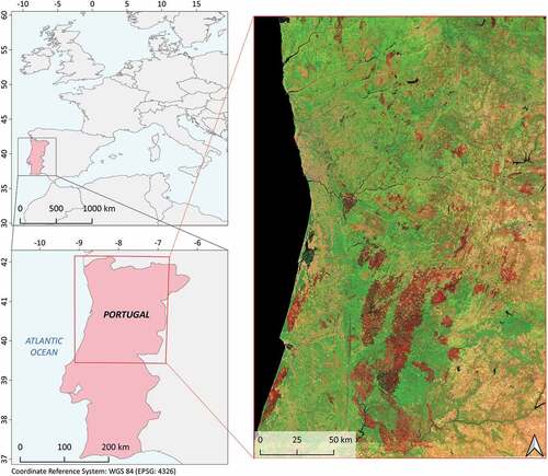
According to statistics provided by the Instituto da Conservaçăo da Natureza e das Florestas (ICNF, 2017), the total burned area from January 1 to October 31 was 442,418 ha. Almost all burned areas (>95% of the national burned surface) occurred inside the present study area. The southern part of Portugal was excluded because it was unaffected by significant events (in terms of the total surface area that affected the country during the fire season analyzed). Only one large fire (defined by ICNF as a fire exceeding 100 ha) occurred outside the study area in southern Portugal.

3. Materials and methods

3.1. Satellite datasets and pre-processing

A multitemporal compositing approach was tested on different progressive fire events in the central and northern parts of Portugal during the fire season in 2017, from June to October. In Mediterranean European regions, this period is considered one of the most severe fire seasons in recent years in terms of the total area burned and environmental and civil damages (San-Miguel-Ayanz et al. 2018). The size of each event was very different, and the spatial distribution over the entire area was considered. Most of the surface (52.37%) was affected during the fire events in October (ICNF, 2017).

Sentinel-2 dataset

The S2 Level-2A (Bottom of the Atmosphere) dataset was preprocessed and downloaded using the Google Earth engine (GEE), which sped up the process considering that most parts of the images are unavailable online in the Copernicus Open Access Hub owing to the long-term policy adopted, which allows only 12 months of the online retention period of the images (Copernicus Long Term Archive Access, 2022).

Focusing on image research in the study area, the first period considered was from June 1 to 15 November 2017. Extending the image search period by a few weeks was necessary so that the number of images covering the last fire season to be analyzed was sufficient. Otherwise, applying the composite criterion could discard the last images of the fire season in which fires could be present. The number of available images for the study area with less than 7.5% cloud cover was 227. After selecting only the red (B4), NIR (B8), and SWIR (B12) bands, the latter was resampled from a 20 m to a 10 m pixel space using bilinear interpolation to relate it to the first two bands. Each of these images was grouped per day of acquisition, and, according to this, a large image mosaic for each acquisition date, covering the entire study area, was produced. The GEE imageCollection.mosaic() function was used for mosaicking.

On some acquisition dates, very few images were taken over the study area; therefore, some mosaics mainly consisted of unavailable pixels. These mosaics were excluded from the final dataset to reduce the time and memory process demand without affecting it. Considering this reduction, the final dataset consisted of three monthly dates, represented by 15 image mosaics for the entire study area (Table 1).

Table 1. Sentinel-2 (S2) and Sentinel-1 (S1) image mosaic dates used in this study (format: year/month/day), acquired before and during the fire season.

Time of acquisition	Sentinel-2 Multispectral Level-2A	Sentinel-1 IW mode Level-1 GRDH
Pre-Fire	2017/04/15	2017/04/14
	2017/04/25	2017/04/20
	2017/04/28	2017/05/02
	2017/05/08	2017/05/14
	2017/05/25	2017/05/26
Fire season	2017/06/04	2017/06/07
	2017/06/07	2017/06/25
	2017/06/24	2017/07/07
	2017/07/07	2017/07/19
	2017/07/14	2017/07/25
	2017/07/24	2017/08/06
	2017/08/03	2017/08/18
	2017/08/13	2017/08/24
	2017/08/23	2017/09/05
	2017/09/02	2017/09/17
	2017/09/12	2017/09/23
	2017/09/22	2017/10/05
	2017/10/02	2017/10/17
	2017/10/22	2017/10/23
	2017/10/26	2017/10/29

As illustrated in the following sections, the change in the detection technique between the pre- and post-fire scenes was implemented to map the burned areas. To do this, a pre-fire composite image was constructed by applying the same pre-processing steps as for the post-fire image, to the images acquired from April 1 to May 31.

Sentinel-1 dataset

The S1 images were downloaded using the Alaska Satellite Facility (ASF) (2022) interface. The S1-A/B high-resolution ground range detected (GRDH), acquired in interferometric wide (IW) mode, and dual-polarized [vertical-horizontal (VH) and vertical-vertical (VV) polarizations] were used. To cover the entire study area, 45 images of the same flight path (path 147, ascending flight direction), consisting of three images for each sensing date (15 sensing dates) and covering the same sensing period adopted for the S2 dataset, were downloaded (Table 1).

The S1 pre-processing workflow commenced by applying precise orbit information and removing thermal noise. This workflow involved radiometric calibration (to beta, β0, nought backscatter standard conventions) (Small 2011) and radiometric terrain correction (RTC) processes, through which the images were radiometrically flattened and geometrically corrected using the shuttle radar topography mission (SRTM) 1 arc-second (Farr et al. 2007) digital elevation model (DEM). All S1 images were mosaicked as a function of the acquisition date, resulting in a final dataset of 15 large image mosaics covering the entire study area, and stacked, relying on the geolocation product to initialize the offset method. A multitemporal Lee filter with a 5 × 5 pixel of window size was employed to reduce the speckle noise (Lee and Pottier 2009). To align each pixel of both datasets, consisting of a 10 m space sampling, the S1 and S2 mosaic datasets were finally stacked, choosing the extent of the S1 dataset as master data for the geolocation and the bilinear as the interpolation method.

3.2. Multitemporal compositing

Optical (Sentinel-2) part

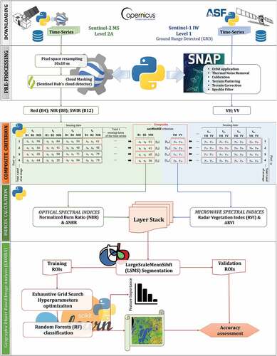
The second lowest NIR composite criterion (secMinNIR) (Figure 2) was adopted in this study for the optical dataset. Considering a time series in which each image corresponds to an acquisition date, each pixel of the final composite image contains the second-lowest value of NIR among the corresponding pixels (exactly aligned xy position in the image) of the entire image time series. For each xy pixel, the process searches for the sensing date where the pixel has the second lowest NIR value.

Figure 2. The flowchart illustrates the second-lowest NIR (secMinNIR) scheme, SAR criteria, and their placement within the workflow.

SAR (Sentinel-1) part

To obtain an SAR composite image, information on the acquisition date of the image to which each pixel of the S2 composite belongs was created, that is, the date when the second lower value of NIR was observed. According to the literature, a fire event does not always correspond to a decrease in the SAR backscatter (Ban et al. 2020; Hosseini and McNairn 2017; Martins et al. 2016; Stroppiana et al. 2015). In the Mediterranean environment, the results depend on different environmental (e.g. humidity and land cover) or sensory (e.g. frequency and polarization) factors (Tanase et al. 2010b, 2010a). This is why a similar compositing approach was not applied to the S1 data. Instead, based on the layer with the date of S2 compositing, for each pixel of the S1 data, the value recorded in the image with the first date of acquisition subsequent to the one corresponding to S2 compositing was chosen. Thus, both the optical and SAR datasets corresponded to information acquired at a similar moment. The S1 and S2 compositing procedure was written in a Python script and could be adapted to be performed on different time frames (monthly, bimonthly, during the entire fire season, etc.). In our case, the criterion was applied for the entire fire season (June-October) and, separately, for the pre-fire period (April-May).

3.3. Object-based burned area mapping

Burned area mapping was carried out by performing supervised object-based geographic object-based image analysis (GEOBIA) classification. The large-scale mean shift (LSMS) algorithm for image segmentation (Michel, Youssefi, and Grizonnet 2015) and random forest (RF) machine learning algorithm for classification (Breiman, 2001; Cutler et al., 2007) were used. The two methods were implemented in Orfeo tool-box v.7.0.0 (OTB) (OTB Homepage, 2021) and Scikit-learn Python library v. 0.23.1 (Pedregosa et al. 2011), respectively.

Input layer creation

From the two optical bands, NIR and SWIR (B8 and B12 bands, respectively), the normalized burn ratio (NBR; eq. 1)(1) $\mathrm{N}\mathrm{B}{\mathrm{R}}_{\mathrm{t}}=\left(\mathrm{N}\mathrm{I}\mathrm{R}-\mathrm{S}\mathrm{W}\mathrm{I}\mathrm{R}\right)/\left(\mathrm{N}\mathrm{I}\mathrm{R}+\mathrm{S}\mathrm{W}\mathrm{I}\mathrm{R}\right)$(1) for the pre- and post-fire periods was computed. From the VH and VV layers, the dual-polarized radar vegetation index (RVI; eq. 2)(2) $\mathrm{R}\mathrm{V}{\mathrm{I}}_{\mathrm{t}}=4\cdot \mathrm{V}\mathrm{H}/\left(\mathrm{V}\mathrm{V}+\mathrm{V}\mathrm{H}\right)$(2) was also calculated for the pre- and post-fire periods. The differences between the post-fire and pre-fire values were computed as ΔNBR (eq. 3)(3) $\mathrm{\Delta }\mathrm{N}\mathrm{B}\mathrm{R}=\mathrm{N}\mathrm{B}{\mathrm{R}}_{\mathrm{p}\mathrm{o}\mathrm{s}\mathrm{t}\mathrm{f}\mathrm{i}\mathrm{r}\mathrm{e}}-\mathrm{N}\mathrm{B}{\mathrm{R}}_{\mathrm{p}\mathrm{r}\mathrm{e}\mathrm{f}\mathrm{i}\mathrm{r}\mathrm{e}}$(3) and ΔRVI (eq. 4)(4) $\mathrm{\Delta }\mathrm{R}\mathrm{V}\mathrm{I}=\mathrm{R}\mathrm{V}{\mathrm{I}}_{\mathrm{p}\mathrm{o}\mathrm{s}\mathrm{t}\mathrm{f}\mathrm{i}\mathrm{r}\mathrm{e}}-\mathrm{R}\mathrm{V}{\mathrm{I}}_{\mathrm{p}\mathrm{r}\mathrm{e}\mathrm{f}\mathrm{i}\mathrm{r}\mathrm{e}}$(4) to allow a change detection approach. Two datasets were created and used as inputs for segmentation and image classification. One was formed by the four layers derived from optical and SAR data (S1+ S2): ΔNBR and post-fire NBR for the optical data, and ΔRVI and post-fire RVI as SAR layers. The second included only two optical layers (S2): ΔNBR and post-fire NBR.

(1) $\mathrm{N}\mathrm{B}{\mathrm{R}}_{\mathrm{t}}=\left(\mathrm{N}\mathrm{I}\mathrm{R}-\mathrm{S}\mathrm{W}\mathrm{I}\mathrm{R}\right)/\left(\mathrm{N}\mathrm{I}\mathrm{R}+\mathrm{S}\mathrm{W}\mathrm{I}\mathrm{R}\right)$(1)

(2) $\mathrm{R}\mathrm{V}{\mathrm{I}}_{\mathrm{t}}=4\cdot \mathrm{V}\mathrm{H}/\left(\mathrm{V}\mathrm{V}+\mathrm{V}\mathrm{H}\right)$(2)

(3) $\mathrm{\Delta }\mathrm{N}\mathrm{B}\mathrm{R}=\mathrm{N}\mathrm{B}{\mathrm{R}}_{\mathrm{p}\mathrm{o}\mathrm{s}\mathrm{t}\mathrm{f}\mathrm{i}\mathrm{r}\mathrm{e}}-\mathrm{N}\mathrm{B}{\mathrm{R}}_{\mathrm{p}\mathrm{r}\mathrm{e}\mathrm{f}\mathrm{i}\mathrm{r}\mathrm{e}}$(3)

(4) $\mathrm{\Delta }\mathrm{R}\mathrm{V}\mathrm{I}=\mathrm{R}\mathrm{V}{\mathrm{I}}_{\mathrm{p}\mathrm{o}\mathrm{s}\mathrm{t}\mathrm{f}\mathrm{i}\mathrm{r}\mathrm{e}}-\mathrm{R}\mathrm{V}{\mathrm{I}}_{\mathrm{p}\mathrm{r}\mathrm{e}\mathrm{f}\mathrm{i}\mathrm{r}\mathrm{e}}$(4)

Before stacking, each layer band was normalized in the same continuous scale range [0–100] (eq. 5)(5) ${\mathrm{X}}_{\mathrm{n}\mathrm{o}\mathrm{r}\mathrm{m}}=\left(\mathrm{X}-{\mathrm{X}}_{\mathrm{m}\mathrm{i}\mathrm{n}}\right)/\left({\mathrm{X}}_{\mathrm{m}\mathrm{a}\mathrm{x}}-{\mathrm{X}}_{\mathrm{m}\mathrm{i}\mathrm{n}}\right)$(5) to equalize and make them comparable as well as reduce the influence of their different scale ranges on the following segmentation process (De Luca, Silva, and Modica 2021, 2019):

(5) ${\mathrm{X}}_{\mathrm{n}\mathrm{o}\mathrm{r}\mathrm{m}}=\left(\mathrm{X}-{\mathrm{X}}_{\mathrm{m}\mathrm{i}\mathrm{n}}\right)/\left({\mathrm{X}}_{\mathrm{m}\mathrm{a}\mathrm{x}}-{\mathrm{X}}_{\mathrm{m}\mathrm{i}\mathrm{n}}\right)$(5)

where X_norm is the normalized value, X is the original value, and X_min and X_max are the lower and highest pixel values of the layer band (original range), respectively.

Image segmentation

The large-scale mean shift (LSMS) is a non-parametric segmentation algorithm introduced by Fukunaga and Hostetler (1975) and developed and improved by Michel, Youssefi, and Grizonnet (2015). It is a tile-based approach, optimized for extensive and/or high-resolution imagery, comprising four successive steps: a) smoothing (filtering), for image noise reduction; b) segmentation, for image subdivision in segments; c) segment merging: for small-size segment reduction; d) vectorization: transformation in vector format, including spectral feature extraction (mean and variance). The first and second steps require setting the two parameters that most influence the final result: range radius and spatial radius. In terms of Euclidean distance, the range radius is the spectral threshold for regrouping two neighboring pixels. The spatial search distance of the neighboring pixels was set based on the spatial radius (measured in the number of pixels). While the spatial radius was set to 25, the range radius was set based on the minimum Euclidean distance between burned and unburned pixels calculated on 300 regions of interest (ROIs) (150 for burned and 150 for unburned areas) scattered over the entire study area. These ROIs, with a size of 4 × 4 pixels, were chosen to cover all the most representative land covers (forest, mainly composed of native Quercus species, Mediterranean Pinus and Eucalyptus plantations; shrublands; pastures; agricultural orchards and crop areas), through visual interpretation supported by several ancillary pieces of information: the high spatial resolution Esri ArcGIS World Imagery map (Esri ArcGIS World Imagery, 2021) and Google Earth Satellite Imagery (Google Earth, 2021), the land use/land cover map of Portugal (Carta de Uso e Ocupação do Solo) (COS, 2018), and the official burned area map of Portugal (ICNF, 2017). The mean value of the pixels in each ROI was computed separately for each optical and/or SAR layer band. The Euclidean distance was calculated for each combined pair of mean ROI values.

The value of the 35^th percentile resulting from the entire Euclidean distance list (composed of each Euclidean distance value between every combination of ROIs) was chosen as the range radius value for the smoothing step. To initialize the segmentation step, the process was repeated on the smoothed images by selecting a series of values around the 10^th percentile of the Euclidean distance list calculated for the smoothed image. To finalize the parameter value set, we carried out a careful trial-and-error procedure to select a suitable range radius value for the segmentation step. The results were visually evaluated at each step of the segmentation process by using a composite optical image of the burned areas. We applied a criterion according to which the burned area was successfully segmented when it was completely “encapsulated” within one or more polygons. There must be no unburned parts in the same polygon. This approach was carried out for both datasets (S1+ S2 and S2), and the final range radius parameter was set as follows: for S1+ S2, 6 (smoothing) and 2 (segmentation); for S2, 12 (smoothing) and 5.8 (segmentation).

In terms of space and radiometry, segments of less than 10 pixels were merged into adjacent segments.

Object-based classification

A well-known RF machine learning algorithm was implemented to classify the segments resulting from the LSMS segmentation. The training polygons were derived by selecting segments that matched the previously selected ROIs used in the segmentation step. In total, 300 training polygons were selected, with 150 for each of the two classes: unburned and burned. The mean (m_s) and variance (v_s) spectral data were used as spectral features to fit and predict the RF model.

The algorithm parameters were set by using the initial out-of-bag (OOB) error estimated by the RF model during the training step as a predictor of the final accuracy level. A set of values was chosen for each RF parameter, and the classification process was initiated for every possible combination of parameter values (Table 2). The combined values that reached the highest OOB were used in the RF model.

Table 2. Parameter values of the random forest (RF) classifier tested through an exhaustive grid search approach to set the optimal combination.

Parameter name	Values set	Description
n_estimators	100, 650, 1200, 1750, 2300, 2850, 3400, 3950, 4500, 5050, 5600, 6150, 6700, 7250, 7800, 8350, 8900, 9450, 10,000	The number of trees in the RF model
max_depth	10, 20, 30, 40, 50, 60, 70, 80, 90, 100, 110, 300, 500, 800, 1000	The maximum depth of the tree
min_samples_split	2, 5, 10	The minimum number of samples required to split an internal node
min_samples_leaf	1, 2, 4	The minimum number of samples required to be at a leaf node
max_features	“auto,” “None,” “log2”	The number of features to consider when looking for the best split

Finally, the Gini feature importance was computed to assess the contribution of each input spectral feature image layer to classification.

3.4. Accuracy assessment

The accuracy assessment was implemented using 1,000 validation sampling points distributed in the study area so that they did not overlap with the training polygons and were labeled following a stratified random approach (Congalton and Green 2019). The official ICNF burned area map was used to initialize stratified sampling, from which 500 points were randomly distributed for each of the two classes (unburned and burned). Subsequently, the distribution of points was optimized through a careful visual assessment supported by the ancillary information already used for the training step (Esri ArcGIS World Imagery, 2021; Google Earth, 2021; COS, 2018) and by each pre- and post-fire Sentinel-2 mosaic image. In addition to avoiding the overlapping of the training polygons, this enabled the improvement of the ICNF map, namely the identification of unburned islands, which were frequently not mapped in the ICNF map. The ICNF maps of the burned area were based on field surveys and complemented with semi-automatic image classification of satellite imagery. Landsat and Sentinel-2 data from 2017 were used (ICNF, 2017). True positive (TP), false negative (FN), and false positive (FP) accuracy categories were computed using the following criteria:

• TP: the sum of burned and unburned corrected classified polygons.

• FP: when an unburned validation polygon corresponds to a polygon classified as burned.

• FN: when a burned validation polygon corresponds to a polygon classified as unburned.

Subsequently, the precision, recall, and F-score accuracy metrics (Equations. 6(6) $precision=\hspace{0.17em}\left|\mathrm{T}\mathrm{P}\right|/\left|\mathrm{T}\mathrm{P}+\mathrm{F}\mathrm{P}\right|$(6) , 7(7) $recall=\hspace{0.17em}\left|\mathrm{T}\mathrm{P}\right|/\left|\mathrm{T}\mathrm{P}+\mathrm{F}\mathrm{N}\right|$(7) , and 8(8) $F-score=\hspace{0.17em}2\cdot \cdot \cdot \hspace{0.17em}precision\cdot \cdot \cdot recall/\hspace{0.17em}\left(precision+recall\right)$(8) ) were computed to evaluate the accuracy of the classified map (Goutte and Gaussier 2005; Shufelt 1999; Sokolova, Japkowicz, and Szpakowicz 2006).

(6) $precision=\hspace{0.17em}\left|\mathrm{T}\mathrm{P}\right|/\left|\mathrm{T}\mathrm{P}+\mathrm{F}\mathrm{P}\right|$(6)

(7) $recall=\hspace{0.17em}\left|\mathrm{T}\mathrm{P}\right|/\left|\mathrm{T}\mathrm{P}+\mathrm{F}\mathrm{N}\right|$(7)

(8) $F-score=\hspace{0.17em}2\cdot \cdot \cdot \hspace{0.17em}precision\cdot \cdot \cdot recall/\hspace{0.17em}\left(precision+recall\right)$(8)

3.5. Spectral separability

Some descriptive statistics of the classified product, namely the total weighted (involving the number of pixels of each polygon) average (µ_sw) and standard deviation (σ_sw) of the values of the spectral feature mean (µ_s) and variance (v_s) of all the resulting polygons, separately for class (burned/unburned), were calculated to further investigate and characterize the resulting output.

The relationship between the differently classified polygons was further analyzed by calculating their spectral separability. The modified M-statistic (Kaufman and Remer 1994) was implemented using the weighted average of the mean values of the spectral polygons (eq. 9)(9) $M-statistic=\hspace{0.17em}\left|{\mu }_1-{\mu }_2\right|/\left({\sigma }_1+{\sigma }_2\right)$(9) :

(9) $M-statistic=\hspace{0.17em}\left|{\mu }_1-{\mu }_2\right|/\left({\sigma }_1+{\sigma }_2\right)$(9)

where µ₁ and µ₂ are the weighted averages of the spectral mean values (µ_sw) for burned and unburned polygons, respectively, and σ₁ + σ₂ are the weighted standard deviations of the spectral mean values (σ_sw) for burned and unburned polygons, respectively. The spectral separability between the two targets increased with an increasing M-statistic.

4. Results

4.1. Optical multitemporal composite image

Figure 3 shows an overview of the multitemporal compositing for the study area and the five illustrative areas. A composite image resulting from the application of the secMinNIR criterion is shown.

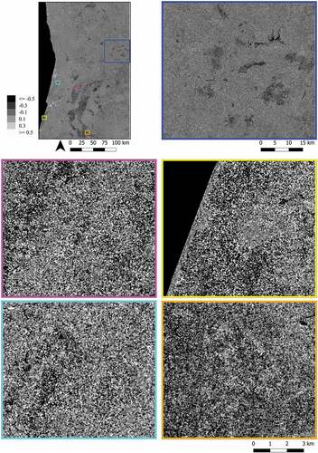
Figure 3. Multitemporal composite output relative to the optical part of the dataset (Sentinel-2) that resulted from processing fire season images (June-October). Five illustrative areas are shown on a more detailed scale beside the overview of the entire study area (top left). The images are shown in RGB combination (R = B12; G = B8; B = B4).

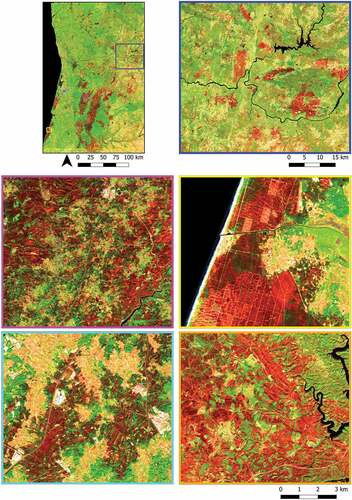
This image consists of Sentinel-2 values observed on the date corresponding to the second-lowest NIR value, considering the time frame from June to October 2017. The RGB image combination (R = B12; G = B8; B = B4) highlights the areas where NIR is lower than the surrounding pixels, making them appear red. These areas are expected to represent the surfaces affected by fire events during the entire fire season.

The destruction of the vegetative part (therefore, of the chlorophyll content) involves a decrease in the reflectance of NIR, followed by a simultaneous increase in red and SWIR; the latter was caused by reduced absorption by water (Miettinen et al. 2013; Pereira et al. 1999). The ΔNBR image, shown in Figure 4, was computed as the difference between the NBR composite image derived for the fire season time series (June–October) by applying the secMinNIR criterion and the NBR image derived for the time series covering the pre-fire period (April–May) by applying the same compositing criterion.

Figure 4. The Figure shows the ΔNBR index map calculated by applying the subtraction NBR_post-fire – NBR_pre-fire. The darker areas correspond to lower index values, while the brighter pixel means represent higher values. The overview of the entire study area is shown on the top-left; five illustrative areas are shown on a more detailed scale.

Using the “post- less pre-fire” formula, the darker areas in the image correspond to lower values of the ΔNBR index, representing a high level of change between the two dates with a decline in NIR and an increase in SWIR.

4.2. SAR multitemporal composite image

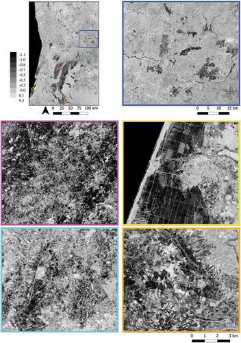
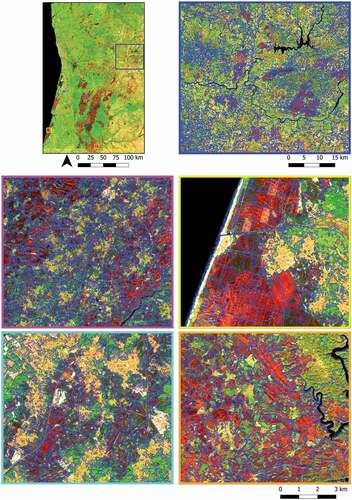
For each optical pixel chosen using the secMinNIR composite criterion, the SAR pixel with the same or the next closest acquisition date was associated with the optical data and used to create a SAR composite image for the same pre- and post-fire periods (April-May and June-October, respectively). The dual-polarized ΔRVI derived from the VH and VV composite SAR images relative to the difference between the pre- and post-fire periods is shown in Figure 5. Considering the gray scalar used in Figure 5, the pixels tend to darken as much as the ΔRVI value is lower, and vice versa.

Figure 5. The ΔRVI index map, calculated by applying the subtraction RVI_post-fire – RVI_pre-fire. The darker areas correspond to lower index values, while the brighter pixels represent higher values. The overview of the entire study area is shown on the top-left; five illustrative areas are shown on a more detailed scale.

The datasets formed by the optical indices (ΔNBR and NBR_post-fire) and SAR indices (ΔRVI and RVI_post-fire) were segmented using the LSMS algorithm. Segmentation was performed on the S1+ S2 and S2 datasets, which resulted in 2,136,807 and 2,238,504 objects, respectively. The area of the objects for the S1+ S2 and S2 datasets ranged from 0.15 ha to 154,969.23 ha (mean = 2.78 ha; standard deviation = 186.40) and from 0.15 ha to 291,812.03 ha (mean = 2.81 ha; standard deviation = 265.98), respectively.

4.3. Segmentation results

The segmentation results for the S1+ S2 and S2 datasets are presented in Figures 6 and 7, respectively. The segments enclose groups of adjacent spectrally homogeneous pixels and, considering only the optical and/or SAR bands sensitive to fire, correspond to the same level of fire severity and are different from the surrounding segments representing burned or not-burned segments.

Figure 6. Segmentation output that resulted from applying the Large-Scale-Mean-Shift (LSMS) algorithm to the S1+ S2 dataset. The segments are presented in a blue border, while the base map is the S2 composite image based on the second-lowest NIR (SecMinNIR) criterion (false-color composite B12-B8-B4). The segmentation is shown for the entire study area (top left) and five detailed illustrative areas.

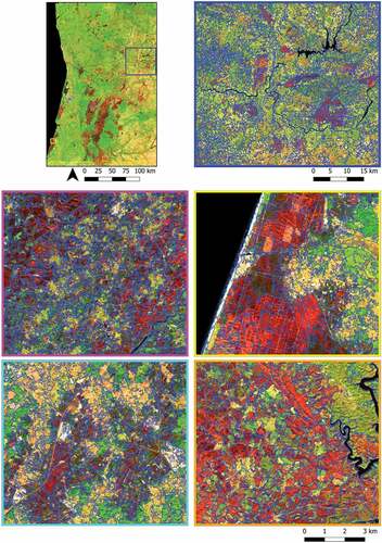
Figure 7. Segmentation output that resulted from applying the Large-Scale-Mean-Shift (LSMS) algorithm to the S2 dataset. The segments are presented in a blue border, while the base map is the S2 composite image based on the second-lowest NIR (SecMinNIR) criterion (false color composite B12-B8-B4). The segmentation is shown for the entire study area (top left) and five detailed illustrative areas.

The unburned part is represented both by most of the study area (unburned surface surrounding the burned areas) and by the small areas not reached by the fire but which are within the burned areas (“unburned islands”). The Figures also show that the transition areas between burned and unburned areas, where the fire caused low-severity damage, were segmented separately from the higher-severity burned areas in both sensor combinations (S1+ S2 and S2).

4.4. GEOBIA classifications and accuracies

Subsequently, the segmented data results were classified using the RF algorithm. The values of the RF parameters, set using the OOB estimated error as a predictive accuracy indicator, are listed in Table 3. As observed, the three parameters did not vary between the two-sensor combinations, maintaining their default original values (min_samples_split:2; min_samples_leaf:1; max_features: “auto”). Reaching an OOB error of 0.924, the set values for n_estimators and max_depth parameters were 1,200 and 110, respectively, using a combination of both sensors (S1+ S2). Using only S2 and an OOB value of 0.908, the values were 1,750 and 65.

Table 3. The final combination of Random Forest (RF) parameter values that resulted from the exhaustive grid search-based test and was used in the classification approach for both datasets (S1+ S2 and S2).

Parameter name	Values (S1+ S2)	Values (S2)
n_estimators	1200	1750
max_depth	110	65
min_samples_split	2	2
min_samples_leaf	1	1
max_features	“auto”	“auto”

The classifications resulting from the GEOBIA process for the S1+ S2 and S2 datasets are shown in Figures 8 and 9, respectively. The images show the segments classified as burned in the entire scene and five representative sample areas. Based on the images, a few differences appear between the sensor combinations. The classified segments encircle the regions affected by the fire. Only a minor confusion is noticeable at the level of some transition areas (e.g. Figures 8–9, bottom left), mainly where the low-severity fire occurred, as observed by comparing the respective ΔNBR maps (Figure 4, bottom left). Some commission errors were also noticeable, involving very small agricultural fields (Figures 8–9, bottom left). The S2 classified map shows that, although it incorporated small transitional areas omitted with the S1+ S2 combination, it made more commission errors by including agricultural and unburned regions adjacent to these areas.

Figure 8. Classification output, based on the S1+ S2 dataset. Segments showing only the burned class (blue) are overlaid on an S2 composite image based on the second-lowest NIR (SecMinNIR) criterion (false color composite B12-B8-B4). The classification is shown for the entire study area (top left) and five detailed illustrative areas.

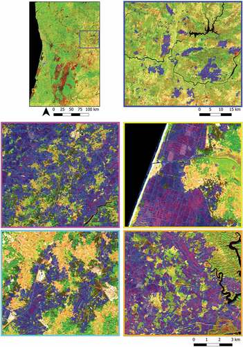
Figure 9. Classification output, based on the S2 dataset. Segments showing only the burned class (blue) are overlaid on an S2 composite image based on the second-lowest NIR (SecMinNIR) criterion (false color composite B12-B8-B4). The classification is shown for the entire study area (top left) and five detailed illustrative areas.

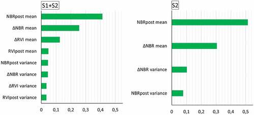
The Gini feature importance was calculated to express the influence of the spectral features (mean and variance) of each image layer during the model prediction process (Figure 10). In both dataset combinations and corresponding burned area classification, the mean spectral feature of NBR_post reached the highest values (0.413 for S1+ S2 and 0.515 for S2), followed by the mean spectral features of ΔNBR (0.256 and 0.305), highlighting the importance of optical data for burned area mapping. When both optical and SAR data were used (S1+ S2), the third and fourth most important features were derived from the SAR data: the mean spectral features of ΔRVI (0.125) and RVI_post (0.048). Below the mean spectral feature importance values, the variance achieved a lower importance value in both dataset combinations, with the lowest absolute variance values reached with the SAR indices (0.035, ΔRVI, and RVI).

Figure 10. Feature importance for burned area mapping (Gini importance), expressed by each spectral feature (mean and variance) used in the classification process for both dataset combinations: S1+ S2 and S2.

The weighted descriptive statistics (µ_sw and σ_sw) calculated for the values of the spectral features (m_s and v_s) of all classified polygons, separately for burned/unburned classes and the image layer, are reported in Table 4. Specifically, only the statistics calculated for the S1+ S2 dataset were reported because the values retrieved for S2 (referable to ΔNBR and NBR) are similar.

Table 4. Weighted descriptive statistics (average, µ_sw; standard deviation, σ_sw), computed using the values of the spectral features (mean, m_s; variance, v_s) of all the classified polygons of each S1+ S2 input layer (ΔNBR, NBR, ΔRVI, RVI), separately for burned and unburned classes.

Image layer	Spectral features	Weighted average (µsw)		Weighted standard deviation (σsw)
		Burned	Unburned	Burned	Unburned
ΔNBR	ms	29.7601	45.8026	4.8992	3.8137
	vs	2.4165	1.4901	2.8745	2.1497
NBR	ms	12.3907	23.8265	2.8068	4.1501
	v^2	1.1457	1.5632	1.9540	1.8859
ΔRVI	ms	47.4288	49.5496	1.7230	1.0755
	v^2	0.8201	0.7188	1.5703	1.5541
RVI	ms	17.5369	20.3481	3.8364	3.9241
	vs	2.6855	3.2240	5.6704	4.2363

As expected, the weighted average of the spectral mean (m_s) for both optical and SAR image layers was higher for the unburned class (45.8026, ΔNBR; 23.8265, NBR; 49.5496, ΔRVI; 20.3481, RVI) than the burned class (29.7601, ΔNBR; 12.3907, NBR; 47.4288, ΔRVI; 17.5369, RVI), and the respective weighted standard deviation was in the range between 1.7230 (ΔRVI) and 4.8992 (ΔNBR) for the burned class, and 1.0755 (ΔRVI) and 4.2363 (RVI) for the unburned class. The second spectral feature, namely the variance (v_s), did not exceed 2.6855 (RVI) and 3.2240 (RVI) for the burned and unburned classes, respectively. The total burned area that occurred during the considered fire season, resulting from classification, was 3,471.75 km² using the S1+ S2 dataset and 3,648.17 km² using the S2 dataset. The accuracy overview of the obtained burned area map was expressed as precision (proportionally inverse to commission errors), recall (proportionally inverse to omission errors), and F-score (representing the overall accuracy of the map). Using the S1+ S2 dataset, the recall, precision, and F-score metrics were 0.954, 0.957, and 0.956, respectively. Using the S2 dataset, the recall, precision, and F-score metrics were 0.969, 0.865, and 0.914, respectively.

5. Discussion

5.1. Image compositing

The final images were composed of all pixels affected by the fire events that occurred during the fire season considered (June–October). This means that all the single events that occurred in the period considered, even in the first month, were potentially equally highlighted in the image. Generally, when a single post-fire image is used to map a long time series of fires, less spectral discrimination of burned areas that occur during the starting and farthest periods of the fire season is expected. This is due to various environmental factors (climatic events, vegetation regrowth, biochemical changes in the burned material, etc.) that could lead to possible confusion with vegetation affected by phenological senescence and/or stress (Dijk et al., 2021; Fraser et al. 2000; Gallagher et al. 2020; Jukka Miettinen et al. 2013; Pereira et al. 1999; Rodman et al. 2021; Verbyla, Kasischke, and Hoy 2008). The high discrimination between burned and unburned areas observed in the composite image is given by the lower NIR reflectance that the vegetation fire induces immediately after the event and in the first few weeks afterward. The minimum NIR values commonly occur on the dates closest to fire extinction. Under these conditions, the difference between the spectral signal from the surrounding background and the discriminability of the burn area was higher. However, choosing the NIR to its minimum value implies that in the final composite, the reflectance values of the surrounding vegetation background are among the lowest in the time series. Cabral et al. (2003) discuss this aspect. However, this makes the image compositing approach less appropriate for some specific applications (e.g. temporal growth monitoring, analysis of the spectral behavior of post-fire vegetation, etc.), the signal reduction is consistent throughout the image, and the relative differences between vegetation types are maintained. This procedure is particularly suitable for qualitative analyses, such as image classification. Choosing a low NIR value ensures that the pixel that best corresponds to the burned area is selected. However, when cloud shadows are present, this involves a substantial reduction in the NIR reflectance on the affected surface, which becomes an obvious problem if we directly choose the pixel with the lowest NIR value, as demonstrated in several studies (Barbosa, Pereira, and Grégoire 1998; Chuvieco et al. 2005; Miettinen and Liew 2008; Pereira et al. 2017, 2016; Sousa, Pereira, and Silva 2003). The same authors demonstrated a method to choose the second-lowest NIR to solve this problem. This is because the strong reduction in optical reflectance caused by cloud shadows has a higher magnitude than that caused by fire. Pereira et al. (2017) showed that the second NIR also overcame the criterion in which the highest SWIR value among the three pixels with the lowest NIR was used. This problem arises when the shadow occupies the same surface twice (or more). The advantage of the latter approach is that SWIR interacts with fire and shadows in a mutually opposite manner. The reflectance values of SWIR increase in the case of vegetation affected by fire because the absorption of electromagnetic waves at these wavelengths by the water is lacking (Pereira et al. 1999). Using ΔNBR boosted the sensitivity of these two bands to the burned vegetation. This well-known index, which is used in burned area mapping, severity estimation, and post-fire monitoring purposes, has been widely explored and its efficacy proven in the literature (Crowley et al. 2019; Donezar et al. 2019; Epting, Verbyla, and Sorbel 2005; Fernández-García et al. 2018; Fornacca, Ren, and Xiao 2018; Key and Benson 2006; Kurum 2015; Miller and Thode 2007; Pulvirenti et al. 2020; Roteta et al. 2019; Schepers et al. 2014; Vanderhoof et al. 2021; Zhang et al. 2019), is also used for the creation of reference maps of burned areas (Ban et al. 2020; De Luca, Silva, and Modica 2021).

Concerning the SAR data on the dual-polarimetric ΔRVI image, the burned areas were visually evident (Figure 5), highlighting the efficiency of the data for visually detecting burned areas. The dual-polarimetric ΔRVI integrates the information of both polarizations (VH and VV), improving the backscatter interception of the variability of volume, structure, and size of the different components of the vegetation canopy and soil (De Luca, Silva, and Modica 2021; Saatchi 2019). The combined contribution of these two elements forms the total SAR signal backscattered from the Earth’s surface, which is covered by vegetation (Saatchi 2019). Cross-polarization presents a higher sensitivity for the distribution of vegetation volume scatterers associated with small branches and leaves. Therefore, it is more efficient in detecting variations in the structure and volume of objects placed on the Earth’s surface, depending on the severity of the disturbance and the length of the wave used (Carreiras et al. 2020; Imperatore et al. 2017; Saatchi 2019; Tanase et al. 2010b). Cross-polarized backscatter tends to decrease when drought conditions persist on the surface (Ruiz-Ramos, Marino, and Boardman 2018). On the other hand, co-polarization intercepts the signal backscattered from the rough surface of bare ground, which is more exposed to the destruction of the canopy after the fire component (Carreiras et al. 2020; Saatchi 2019).

5.2. GEOBIA application

Several studies have successfully applied GEOBIA to map burned areas for mapping purposes (Gitas, Mitri, and Ventura 2004; Mitri and Gitas 2004; Polychronaki and Gitas 2010, 2012; Sertel and Alganci 2016; Shimabukuro et al. 2015) as an alternative classification technique to the pixel-based approach, observing that the former mitigates common biases provided by the pixel-based approach. Georgopoulos, Stavrakoudis, and Gitas (2019) presented an OBIA methodology based on mean-shift and support vector machine (SVM) algorithms for segmentation and classification, respectively, to map burned areas using Sentinel-2 data. The advantage of the GEOBIA approach is that, using the average value of the set of pixels contained within a segment, instead of any single value, the pixel variance caused by possible outliers is reduced, increasing the reliability of the classification (Radoux and Defourny 2008). Considering only the spectral mean pixel value of the objects is a more efficient approach in the case of SAR data where, even if the speckle filter is applied, speckle noise remains in the images (Polychronaki et al. 2013). The integration of both spectral features used in the present work (mean and variance) was thus expected to provide an advantage in classifying the two burned/unburned binary classes as additional information on the variability of the objects inside the polygons compared with using only the mean. However, the importance of the resulting features demonstrated that the former feature was not as decisive as the spectral mean for both optical and SAR data. This was because the spectral separability expressed by the mean was sufficiently discriminatory Table 5. An M-statistic higher than 1 means that the discrimination is relatively strong (De Luca et al. 2019; Kaufman and Remer 1994). Furthermore, the weighted statistics (Table 4) demonstrated that the variance did not differ significantly between the burned and unburned classes.

A combination of uncorrelated feature spaces (e.g. shape and topological features) is considered to be able to avoid classification confusion and improve accuracy (Gitas, Mitri, and Ventura 2004; Mitri and Gitas 2004; Polychronaki et al. 2013; Polychronaki and Gitas 2010).

5.3. Map accuracy

The classification accuracy assessment results reached high levels in both cases (S1+ S2 and S2), as represented by an F-score value of more than 0.9. Although there was an effective distinction between most agricultural areas (plowed fields) and burned areas, some commission errors distributed over the entire study area remained when only an optical dataset was used. Tillage exposed the underlying soil layers on the surface, eliminating the vegetation present and causing a spectral response in some cases comparable to that caused by a low-severity fire (Dijk et al., 2021). When ΔNBR was used, which was the most “important” layer for the learning model (Figure 10), the spectral separability was indeed higher between agricultural fields and unburned polygons than between the former and the burned surface (Table 6). However, the extent of these errors remained low, considering the size of the study area and minimal amount of spectral information used. Conversely, SAR achieved low separability in all cases (<1). Separability was sufficiently high if agricultural fields were compared with the burned class and when using the SAR layer with the highest importance in the RF learning process. Speckle noise may also play a dual role in this issue. Even after the filtering process, the SAR image layers presented persistent speckle outliers (Figure 5) owing to the intrinsic characteristics of the SAR signal (De Luca, Silva, and Modica 2021). At smaller scales (such as those of agricultural fields), this implies higher mixing with the background (Figure 5, bottom left). This could decrease the distinguishability of agricultural fields and affect small burned areas or transition areas between burned and unburned areas (Figure 5, bottom left). However, this would be relevant when using only SAR data, rather than integrating both optical and SAR information. Several studies (De Luca, Silva, and Modica 2021; Polychronaki et al. 2013; Verhegghen et al. 2016) have addressed false positives and negatives using only SAR-based datasets caused by either the strong influence of moisture changes in bare soil or speckle noise. Considering the results of the present study, the feature importance demonstrates how the SAR product contributes to the final accuracy at a lower level than the optical product. However, the accuracy results indicate that the integrated use of optical and SAR datasets reduces commission errors, correcting the erroneous identification of burned areas that could occur using individual types of sensors, as already observed in Stroppiana et al. (2015). This confirms what other authors have considered using SAR as complementary data, rather than a substitute for optical data (De Luca, Silva, and Modica 2021; Lasko 2019; Lehmann et al. 2015; Polychronaki et al. 2013; Stroppiana et al. 2015). Optical sensors are more effective for burned area mapping because of the more robust relationship between the optical wavelengths and the effects of fire on vegetation.

However, SAR data are fundamental not only for proven complementary information that improves classification, but also for fire detection in unfavorable atmospheric conditions, owing to the ability of microwaves to penetrate cloud cover (Richards 2009). However, this latter aspect is less important in the Mediterranean climate context than in the tropical zone.

5.4. Final considerations and limitations

Burned area maps, covering regional to continental/global territory, derived from coarse and medium spatial resolution satellite sensors (e.g. NASA Terra/Aqua MODIS, SPOT-VEGETATION, NOAA/AVHRR) have certainly been an important source of information for the fire science and application communities (Boschetti et al. 2015). As demonstrated in this and other studies, the free availability of Sentinel satellites with enhanced spatial and temporal resolution offers new opportunities that guarantee the fast distribution of burned area products at very high accuracy and large scales. This can only be achieved if all fire events, including small fires (between 0.1 and 1 km²), and small unburned islands are detected. The use of improved spatial resolutions guarantees more precise monitoring, even within the same burned areas, because all the details (e.g. unburned spots) can be surveyed. The increase in time and processing consumption required by higher resolution is also overcome by the development of open-source software solutions and cloud platforms that allow the easy processing of large amounts of data (Chuvieco et al. 2019).

The findings of this approach open a debate regarding the quality of official reference data. Official maps based on coarse data tend to overestimate burned areas. They fail to classify many unburned islands, rendering the produced map almost unusable as a reference. In our case, this problem was overcome by integrating freely available high-resolution images with accurate visual analysis. However, in our opinion, this method is laborious. For this reason, there is a need for increasingly accurate mapping methods for relatively large territories (and/or specific fire seasons) that lack accurate maps of burned areas.

The results of this study showed that using only the NIR and SWIR bands, already known to be the most sensitive bands for discriminating burned areas (Chuvieco et al. 2005; Pereira et al. 1999), with or without the integrated use of given SAR, it is possible to achieve high values of accurate burned area mapping quality (accuracy >90%). This is an essential aspect favoring a more rapid and effective practical operability of the approach.

Although the integration of the SAR data slightly increased the accuracy, it did not overcome the importance expressed by the information of the optical indices during the learning process.

Although this was not the case in this study, the method might be hindered by the frequent presence of cloud shadows on the same pixels, which is typical in more temperate European climates. The advantages of SAR should be investigated and possibly raised in these cases. Integrating the highest SWIR (Pereira et al. 2017) might be another valid solution, considering the already addressed weaknesses compared with the secMinNIR.

6. Conclusions and recommendations

The objective of this study was to optimize a method of detecting burned areas that occurred during an entire fire season, based on a multitemporal compositing criterion and image segmentation, through the integration of optical and SAR data, open-source software, and algorithms. This study contributes to the development and harmonization of accurate methods used for the detection of burned areas at national and continental levels. These objectives were pursued based on the robustness and spatial adaptability of the algorithm. The approach was tested and validated on a large regional scale in a heterogeneous Mediterranean territory with fire conditions of varying severity and different burned vegetation and temporal progression. We believe that this method could be extended to other European ecosystems. Future studies might involve verifying the performance of the proposed classification workflow in other Mediterranean regions or ecosystems. However, the efficiency of SAR information when cloud shadows occupy the same pixel for more scenes should be tested and compared, especially in more temperate climates, as should the eventual integration of the highest SWIR value into the composite process.

Our findings suggest that optical data can only achieve high levels of accuracy. However, optical and SAR imagery synergy can improve the accuracy of burned-area mapping. Despite this, we believe that optical data alone can be used as the first effective solution for the detection of burned vegetation areas, allowing easier data management and less time-consuming processing. These aspects are fundamental in operational scenarios in which disaster mapping methodologies such as fires are used. The utilization of other bands, frequencies, polarization combinations, or indices may provide improvements for further analysis. In particular, many optical indices have been implemented and proposed as optimized for the detection of burned areas compared to standard NBR [e.g. BAIS2 (Filipponi 2018) or the recent NBR+ (Alcaras et al. 2022)]. Supplementary analyses should integrate, test, and compare these data to optimize the approach proposed in this study further.

Further optimizations might entail using open-source cloud computing platforms, such as the Google Earth Engine (GEE), where an extensive database of satellite imagery and computational power is accessible to all users.

Acknowledgements

The authors would thank Duarte Oom (European Joint Research Group, JRC, Ispra; Instituto Superior de Agronomia, University of Lisbon, Lisbon) for making its JavaScript-based optical data-based compositing algorithm available, helpful in initializing the early stages of work.

Disclosure statement

No potential conflict of interest was reported by the author(s).

Data availability statement

The data supporting this study’s findings are available from the corresponding author upon reasonable request. These data were derived from the following resources available in the public domain: ESA Sentinel Homepage (2021).

Additional information

Funding

Giandomenico De Luca was funded by the European Commisison and the Regione Calabria with the POR Calabria FESR FSE 2014-2020source [CUP C39B18000070002]. João M. N. Silva was funded by the Forest Research Centre, a research unit funded by Fundação para a Ciência e a Tecnologia I.P. (FCT), Portugal (UIDB/00239/2020), and by the project FireCast - Forecasting fire probability and characteristicsfor a habitable pyroenvironment, funded by FCT (PCIF/GRF/0204/2017).

References

- Alcaras, E., D. Costantino, F. Guastaferro, C. Parente, and M. Pepe. 2022. “Normalized Burn Ratio Plus (NBR+): A New Index for Sentinel-2 Imagery.” Remote Sensing 14 (7): 1727. doi:10.3390/rs14071727.
- ASF. 2022. Accessed July 21. https://asf.alaska.edu/.
- Axel, A. C., 2018. Burned Area Mapping of an Escaped Fire into Tropical Dry Forest in Western Madagascar Using Multi-Season Landsat OLI Data. Remote Sens. https://doi.org/10.3390/rs10030371
- Ban, Y., P. Zhang, A. Nascetti, A. R. Bevington, and M. A. Wulder. 2020. “Near Real-Time Wildfire Progression Monitoring with Sentinel-1 SAR Time Series and Deep Learning.” Scientific Reports 10 (1): 1–15. doi:10.1038/s41598-019-56967-x.
- Barbosa, P. M., J. M. C. Pereira, and J.-M. Grégoire. 1998. “Compositing Criteria for Burned Area Assessment Using Multitemporal Low Resolution Satellite Data.” Remote Sensing of Environment 65 (1): 38–49.
- Barbosa, P. M., D. Stroppiana, J. M. Grégoire, and J. M. C. Pereira. 1999. “An Assessment of Vegetation Fire in Africa (1981-1991): Burned Areas, Burned Biomass, and Atmospheric Emissions.” Global Biogeochemical Cycles 13 (4): 933–950. doi:10.1029/1999GB900042.
- Belenguer-Plomer, M. A., E. Chuvieco, and M. A. Tanase. 2019. “Temporal Decorrelation of C-Band Backscatter Coefficient in Mediterranean Burned Areas.” Remote Sensing 11 (22): 2661. doi:10.3390/rs11222661.
- Boschetti, L., D. P. Roy, C. O. Justice, and M. L. Humber. 2015. “MODIS–Landsat Fusion for Large Area 30m Burned Area Mapping.” Remote Sens. Environ 161: 27–42. doi:10.1016/j.rse.2015.01.022.
- Breiman L. 2001. Machine Learning. 45(1): 5–32. doi:10.1023/A:1010933404324
- Cabral, A., M. J. P. De Vasconcelos, J. M. C. Pereira, É. Bartholomé, and P. Mayaux. 2003. “Multi-temporal Compositing Approaches for SPOT-4 Vegetation.” International Journal of Remote Sensing 24 (16): 3343–3350. doi:10.1080/0143116031000075936.
- Carreiras, J. M. B., S. Quegan, K. Tansey, and S. Page. 2020. “Sentinel-1 Observation Frequency Significantly Increases Burnt Area Detectability in Tropical SE Asia.” Environmental Research Letters 15 (5): 054008. doi:10.1088/1748-9326/ab7765.
- Cascio, W. E. 2018. “Wildland Fire Smoke and Human Health.” The Science of the Total Environment 624: 586–595. doi:10.1016/j.scitotenv.2017.12.086.
- Christopoulou, A., N. M. Fyllas, P. Andriopoulos, N. Koutsias, P. G. Dimitrakopoulos, and M. Arianoutsou. 2014. “Post-fire Regeneration Patterns of Pinus Nigra in a Recently Burned Area in Mount Taygetos, Southern Greece: The Role of Unburned Forest Patches.” Forest Ecology and Management 327: 148–156. doi:10.1016/j.foreco.2014.05.006.
- Chuvieco, E. 2009. “Earth Observation of Wildland Fires in Mediterranean Ecosystems, Earth Observation of Wildland Fires in Mediterranean Ecosystems.” Springer Berlin Heidelberg. doi:10.1007/978-3-642-01754-4.
- Chuvieco, E., and M. P. Martin. 1994. “Global Fire Mapping and Fire Danger Estimation Using AVHRR Images.” Photogramm. Eng. Remote Sensing 60: 563–570.
- Chuvieco, E., F. Mouillot, G. R. van der Werf, J. San Miguel, M. Tanasse, N. Koutsias, M. García, et al. 2019. “Historical Background and Current Developments for Mapping Burned Area from Satellite Earth Observation.” Remote Sens. Environ 225: 45–64. doi:10.1016/j.rse.2019.02.013.
- Chuvieco, E., G. Ventura, M. P. Martín, and I. Gómez. 2005. “Assessment of Multitemporal Compositing Techniques of MODIS and AVHRR Images for Burned Land Mapping.” Remote Sensing of Environment 94 (4): 450–462. doi:10.1016/j.rse.2004.11.006.
- Chuvieco, E., C. Yue, A. Heil, F. Mouillot, I. Alonso-Canas, M. Padilla, J. M. Pereira, D. Oom, and K. Tansey. 2016. “A New Global Burned Area Product for Climate Assessment of Fire Impacts.” Global Ecology and Biogeography 25 (5): 619–629. doi:10.1111/geb.12440.
- Congalton, R. G., and K. Green, 2019. Assessing the Accuracy of Remotely Sensed Data. Principles and Practices, CRC Press
- Copernicus Long Term Archive Access. 2022. Accessed July 21. https://scihub.copernicus.eu/userguide/LongTermArchive
- COS. 2018. Accessed July 21 2012. https://www.dgterritorio.gov.pt/Carta-de-Uso-e-Ocupacao-do-Solo-para-2018
- Crowley, M. A., J. A. Cardille, J. C. White, and M. A. Wulder. 2019. “Generating intra-year Metrics of Wildfire Progression Using Multiple open-access Satellite Data Streams.” Remote Sens. Environ 232: 111295. doi:10.1016/j.rse.2019.111295.
- Cutler D. R., T. C. Edwards, K. H. Beard, A. Cutler, K. T. Hess, J. Gibson and J. J. Lawler. 2007. “Random Forests for Classification in Ecology.“ Ecology 88 (11): 2783–2792. doi:10.1890/07-0539.1
- De Luca, G., N. Silva, J. M. Cerasoli, S. Araújo, J. Campos, J. Di Fazio, and S. Modica, G. 2019. “Object-Based Land Cover Classification of Cork Oak Woodlands Using UAV Imagery and Orfeo ToolBox.” Remote Sensing 11 (10): 1238. doi:10.3390/rs11101238.
- De Luca, G., J. M. N. Silva, and G. Modica. 2021. “A Workflow Based on Sentinel-1 SAR Data and open-source Algorithms for Unsupervised Burned Area Detection in Mediterranean Ecosystems.” GIScience Remote Sens 00: 1–26. doi:10.1080/15481603.2021.1907896.
- Donezar, U., T. De Blas, A. Larrañaga, F. Ros, L. Albizua, A. Steel, and M. Broglia. 2019. “Applicability of the Multitemporal Coherence Approach to Sentinel-1 for the Detection and Delineation of Burnt Areas in the Context of the Copernicus Emergency Management Service.” Remote Sensing 11 (22): 2607. doi:10.3390/rs11222607.
- EFFIS Annual Fire Reports. 2021. Accessed May 04. https://effis.jrc.ec.europa.eu/reports-and-publications/annual-fire-reports
- EFFIS Rapid Damage Assessment. 2021. Accessed September 26. https://effis.jrc.ec.europa.eu/about-effis/technicavl-background/rapid-damage-assessment
- Epting, J., D. Verbyla, and B. Sorbel. 2005. “Evaluation of Remotely Sensed Indices for Assessing Burn Severity in Interior Alaska Using Landsat TM and ETM+.” Remote Sensing of Environment 96 (3–4): 328–339. doi:10.1016/j.rse.2005.03.002.
- ESA Sentinel Homepage. 2021. Accessed March 11. https://sentinel.esa.int/web/sentinel/home
- Esri ArcGIS World Imagery. 2021. Accessed March 19. https://www.arcgis.com/home/item.html?id=10df2279f9684e4a9f6a7f08febac2a9
- European Environment Agency. 2021. Accessed July 21. https://www.eea.europa.eu/data-and-maps/daviz/burnt-forest-area-in-five-3/#tab-chart_5
- Eva, H., and E. F. Lambin. 1998. “Burnt Area Mapping in Central Africa Using ATSR Data.” International Journal of Remote Sensing 19 (18): 3473–3497. doi:10.1080/014311698213768.
- Farr, T. G., P. A. Rosen, E. Caro, R. Crippen, R. Duren, S. Hensley, M. Kobrick, et al. 2007. “The Shuttle Radar Topography Mission.” Reviews of Geophysics 45 (2): 1–33. doi:10.1029/2005RG000183.
- Fernández-García, V., M. Santamarta, A. Fernández-Manso, C. Quintano, E. Marcos, and L. Calvo. 2018. “Burn Severity Metrics in fire-prone Pine Ecosystems along a Climatic Gradient Using Landsat Imagery.” Remote Sens. Environ 206: 205–217. doi:10.1016/j.rse.2017.12.029.
- Fernández, A., P. Illera, and J. L. Casanova. 1997. “Automatic Mapping of Surfaces Affected by Forest Fires in Spain Using AVHRR NDVI Composite Image Data.” Remote Sens. Environ 60 (2): 153–162. doi:10.1016/S0034-4257(96).
- Filipponi, F. 2018. “BAIS2: Burned Area Index for Sentinel-2.” Proceedings 5177. doi:10.3390/ecrs-2-05177.
- Filipponi, F. 2019. “Exploitation of Sentinel-2 Time Series to Map Burned Areas at the National Level: A Case Study on the 2017 Italy Wildfires.” Remote Sensing 11 (6): 622. doi:10.3390/rs11060622.
- Fornacca, D., G. Ren, and W. Xiao. 2018. “Evaluating the Best Spectral Indices for the Detection of Burn Scars at Several post-fire Dates in a Mountainous Region of Northwest Yunnan, China.” Remote Sensing 10 (8): 1196. doi:10.3390/rs10081196.
- Fraser, R. H., Z. Li, J. Cihlar, Z. Li, J. Cihlar, and J. Cihlar. 2000. “Hotspot and NDVI Differencing Synergy (HANDS): A New Technique for Burned Area Mapping over Boreal Forest.” Remote Sensing of Environment 74 (3): 362–376. doi:10.1016/S0034-4257(00).
- Fukunaga, K., and L. D. Hostetler. 1975. “The Estimation of the Gradient of a Density Function, with Applications in Pattern Recognition.” IEEE Transactions on Information Theory 21 (1): 32–40. doi:10.1109/TIT.1975.1055330.
- Gallagher, M. R., N. S. Skowronski, M. R. Gallagher, N. S. Skowronski, E. J. Green, R. G. Lathrop, E. J. Green, et al. 2020. “An Improved Approach for Selecting and Validating Burn Severity Indices in Forested Landscapes an Improved Approach for Selecting and Validating Burn Severity Indices in Feux Dans Des Milieux Forestiers.” . Canadian Journal of Remote Sensing 46 (1): 100–111. doi:10.1080/07038992.2020.1735931.
- Georgopoulos, N., D. Stavrakoudis, and I. Z. Gitas, 2019. Object-Based Burned Area Mapping Using Sentinel-2 Imagery and Supervised Learning Guided by Empirical Rules in: IGARSS 2019-2019 IEEE International Geoscience and Remote Sensing Symposium, 28 July - 2 August 2019, Yokohama, Japan, pp. 9980–9983. 10.1109/IGARSS.2019.8900134
- Giglio, L., L. Boschetti, D. P. Roy, M. L. Humber, and C. O. Justice. 2018. “The Collection 6 MODIS Burned Area Mapping Algorithm and Product.” Remote Sens. Environ 217: 72–85. doi:10.1016/j.rse.2018.08.005.
- Gimeno, M., J. San-Miguel-Ayanz, and G. Schmuck. 2004. “Identification of Burnt Areas in Mediterranean Forest Environments from ERS-2 SAR Time Series.” International Journal of Remote Sensing 25 (22): 4873–4888. doi:10.1080/01431160412331269715.
- Gitas, I. Z., G. H. Mitri, and G. Ventura. 2004. “Object-based Image Classification for Burned Area Mapping of Creus Cape, Spain, Using NOAA-AVHRR Imagery.” Remote Sensing of Environment 92 (3): 409–413. doi:10.1016/j.rse.2004.06.006.
- Gitas, I., G. Mitri, S. Veraverbeke, and A. Polychronaki. 2012. “Advances in Remote Sensing of Post-Fire Vegetation Recovery Monitoring - A Review.” Remote Sens. Biomass - Princ. Appl. doi:10.5772/20571.
- Goodwin, N. R., and L. J. Collett. 2014. “Development of an Automated Method for Mapping Fire History Captured in Landsat TM and ETM+ Time Series across Queensland, Australia.” Remote Sens. Environ 148: 206–221. doi:10.1016/j.rse.2014.03.021.
- Google Earth. 2021. Accessed March 19. https://www.google.com/earth/index.html
- Goutte, C., and E. Gaussier. 2005. “A Probabilistic Interpretation of Precision, Recall and F-Score, with Implication for Evaluation.” Lect. Notes Comput. Sci 3408: 345–359. doi:10.1007/978-3-540-31865-1_25.
- Hachani, A., M. Ouessar, S. Paloscia, E. Santi, and S. Pettinato. 2019. “Soil Moisture Retrieval from Sentinel-1 Acquisitions in an Arid Environment in Tunisia: Application of Artificial Neural Networks Techniques.” International Journal of Remote Sensing 40 (24): 9159–9180. doi:10.1080/01431161.2019.1629503.
- Hardy, C. C. 2005. “Wildland Fire Hazard and Risk: Problems, Definitions, and Context.” Forest Ecology and Management 211 (1–2): 73–82. doi:10.1016/j.foreco.2005.01.029.
- Hawbaker, T. J., M. K. Vanderhoof, Y.-J. Beal, J. D. Takacs, G. L. Schmidt, J. T. Falgout, B. Williams, et al. 2017. “Mapping Burned Areas Using Dense time-series of Landsat Data.” Remote Sensing of Environment 198: 504–522. doi:10.1016/j.rse.2017.06.027.
- Holben, B. N. 1986. “Characteristics of maximum-value Composite Images from Temporal AVHRR Data.” International Journal of Remote Sensing 7 (11): 1417–1434. doi:10.1080/01431168608948945.
- Hosseini, M., and H. McNairn. 2017. “Using multi-polarization C- and L-band Synthetic Aperture Radar to Estimate Biomass and Soil Moisture of Wheat Fields.” Int. J. Appl. Earth Obs. Geoinf 58: 50–64. doi:10.1016/j.jag.2017.01.006.
- ICNF. 2017. Accessed May 18. https://www.icnf.pt/api/file/doc/2c45facee8d3e4f8
- Imperatore, P., R. Azar, F. Calo, D. Stroppiana, P. A. Brivio, R. Lanari, and A. Pepe. 2017. “Effect of the Vegetation Fire on Backscattering: An Investigation Based on Sentinel-1 Observations.” IEEE Journal of Selected Topics in Applied Earth Observations and Remote Sensing 10 (10): 4478–4492. doi:10.1109/JSTARS.2017.2717039.
- Inoue, Y., J. Qi, A. Olioso, Y. Kiyono, T. Horie, H. Asai, K. Saito, et al. 2008. “Reflectance characteristics of major land surfaces in slash‐and‐burn ecosystems in Laos.” International Journal of Remote Sensing 29 (7): 2011–2019. doi:10.1080/01431160701442039.
- Kasischke, E. S., N. H. F. French, P. Harrell, N. L. Christensen, S. L. Ustin, and D. Barry. 1993. “Monitoring of Wildfires in Boreal Forests Using Large Area AVHRR NDVI Composite Image Data.” Remote Sensing of Environment 45 (1): 61–71. doi:10.1016/0034-4257(93).
- Kaufman, Y. J., and L. A. Remer. 1994. “Detection of Forests Using Mid-IR Reflectance: An Application for Aerosol Studies.” IEEE Transactions on Geoscience and Remote Sensing 32 (3): 672–683. doi:10.1109/36.297984.
- Key, C. H., and N. C. Benson, 2006. Landscape Assessment (LA) Sampling and Analysis Methods, In: FIREMON: Fire Effects Monitoring and Inventory System
- Kim, Y., T. Jackson, R. Bindlish, S. Hong, G. Jung, and K. Lee. 2014. “Retrieval of Wheat Growth Parameters with Radar Vegetation Indices.” IEEE Geoscience and Remote Sensing Letters 11 (4): 808–812. doi:10.1109/LGRS.2013.2279255.
- Kim, Y., T. Jackson, R. Bindlish, H. Lee, and S. Hong. 2012. “Radar Vegetation Index for Estimating the Vegetation Water Content of Rice and Soybean.” IEEE Geoscience and Remote Sensing Letters 9 (4): 564–568. doi:10.1109/LGRS.2011.2174772.
- Kim, Y., and J. J. Van Zyl. 2009. “A time-series Approach to Estimate Soil Moisture Using Polarimetric Radar Data.” IEEE Trans. Geosci. Remote Sens. doi:10.1109/TGRS.2009.2014944.
- Knopp, L., M. Wieland, M. Rättich, and S. Martinis. 2020. “A Deep Learning Approach for Burned Area Segmentation with Sentinel-2 Data.” Remote Sensing 12 (15): 2422. doi:10.3390/RS12152422.
- Kurum, M., 2015. C-Band SAR Backscatter Evaluation of 2008 Gallipoli Forest Fire 12, 1091–1095.
- Lasaponara, R., and B. Tucci. 2019. “Identification of Burned Areas and Severity Using SAR Sentinel-1.” IEEE Geoscience and Remote Sensing Letters 16 (6): 917–921. doi:10.1109/LGRS.2018.2888641.
- Lasko, K. 2019. “Incorporating Sentinel-1 SAR Imagery with the MODIS MCD64A1 Burned Area Product to Improve Burn Date Estimates and Reduce Burn Date Uncertainty in Wildland Fire Mapping Incorporating Sentinel-1 SAR Imagery with the MODIS MCD64A1 Burned Area Product to Imp.” Geocarto International 0: 1–21. doi:10.1080/10106049.2019.1608592.
- Lee, J.-S., and E. Pottier. 2009. “Filtering of Single Polarization SAR Data, In: CRC Press. (Ed.), Polarimetric Radar Imaging. From Basics to Applications.” CRC Press., Boca Raton. doi:10.1201/9781420054989.
- Lehmann, E. A., P. Caccetta, K. Lowell, A. Mitchell, Z.-S. Zhou, A. Held, T. Milne, and I. Tapley. 2015. “SAR and Optical Remote Sensing: Assessment of Complementarity and Interoperability in the Context of a large-scale Operational Forest Monitoring System.” Remote Sensing of Environment 156: 335–348. doi:10.1016/j.rse.2014.09.034.
- Llorens, R., J. A. Sobrino, C. Fernández, J. M. Fernández-Alonso, and J. A. Vega. 2021. “A Methodology to Estimate Forest Fires Burned Areas and Burn Severity Degrees Using Sentinel-2 Data. Application to the October 2017 Fires in the Iberian Peninsula. Int. J. Appl. Earth Obs.” Geoinf 95: 102243. doi:10.1016/j.jag.2020.102243.
- Martins, F. S. R. V., J. R. Dos Santos, L. S. Galvao, and H. A. M. Xaud. 2016. “Sensitivity of ALOS/PALSAR Imagery to Forest Degradation by Fire in Northern Amazon.” Int. J. Appl. Earth Obs. Geoinf 49: 163–174. doi:10.1016/j.jag.2016.02.009.
- Mayaux, P., V. Gond, and E. Bartholome. 2000. “A near-real Time forest-cover Map of Madagascar Derived from SPOT-4 VEGETATION Data.” International Journal of Remote Sensing 21 (16): 3139–3144. doi:10.1080/01431160050145018.
- Meddens, A. J. H., C. A. Kolden, and J. A. Lutz. 2016. “Detecting Unburned Areas within Wildfire Perimeters Using Landsat and Ancillary Data across the Northwestern United States.” Remote Sensing of Environment 186: 275–285. doi:10.1016/j.rse.2016.08.023.
- Michel, J., D. Youssefi, and M. Grizonnet. 2015. “Stable Mean-Shift Algorithm and Its Application to the Segmentation of Arbitrarily Large Remote Sensing Images.” IEEE Transactions on Geoscience and Remote Sensing 53 (2): 952–964. doi:10.1109/TGRS.2014.2330857.
- Miettinen, J., E. Hyer, A. S. Chia, L. K. Kwoh, and S. C. Liew. 2013. “Detection of Vegetation Fires and Burnt Areas by Remote Sensing in Insular Southeast Asian Conditions: Current Status of Knowledge and Future Challenges.” International Journal of Remote Sensing 34 (12): 4344–4366. doi:10.1080/01431161.2013.777489.
- Miettinen, J., and S. C. Liew. 2008. “Comparison of Multitemporal Compositing Methods for Burnt Area Detection in Southeast Asian Conditions.” International Journal of Remote Sensing 29 (4): 1075–1092. doi:10.1080/01431160701281031.
- Miller, J. D., and A. E. Thode. 2007. “Quantifying Burn Severity in a Heterogeneous Landscape with a Relative Version of the Delta Normalized Burn Ratio (Dnbr).” Remote Sensing of Environment 109 (1): 66–80. doi:10.1109/LGRS.2011.2174772.
- Mitri, G. H., and I. Z. Gitas. 2004. “A semi-automated object-oriented Model for Burned Area Mapping in the Mediterranean Region Using Landsat-TM Imagery.” International Journal of Wildland Fire 13 (3): 367–376. doi:10.1109/LGRS.2018.2888641.
- Mpakairi, K. S., H. Ndaimani, and B. Kavhu. 2020. “Exploring the Utility of Sentinel-2 MSI Derived Spectral Indices in Mapping Burned Areas in Different land-cover Types.” Scientific African 10: e00565. doi:10.1016/j.rse.2016.08.023.
- Navarro, G., I. Caballero, G. Silva, P.-C. Parra, Á. Vázquez, and R. Caldeira. 2017. “Evaluation of Forest Fire on Madeira Island Using Sentinel-2A MSI Imagery.” Int. J. Appl. Earth Obs. Geoinf 58: 97–106. doi:10.1016/j.jag.2017.02.003.
- OTB Homepage. 2021. Accessed March 19. https://www.orfeo-toolbox.org/
- Otón, G., R. Ramo, J. Lizundia-Loiola, and E. Chuvieco. 2019. “Global Detection of long-term (1982-2017) Burned Area with AVHRR-LTDR Data.” Remote Sensing 11 (18): 2079. doi:10.3390/rs11182079.
- Pedregosa, F., G. Varoquaux, A. Gramfort, V. Michel, B. Thirion, O. Grisel, M. Blondel, et al. 2011. “Scikit-learn: Machine Learning in Python.” Journal of Machine Learning Research 12: 2825–2830.
- Pepe, A., D. Stroppiana, F. Calo, P. Imperatore, L. Boschetti, C. Bignami, and P. A. Brivio. 2018. “Exploitation of Copernicus Sentinels Data for Sensing Fire-Disturbed Vegetated Areas.“ IGARSS 2018 - 2018 IEEE International Geoscience and Remote Sensing Symposium, 22-27 July 2018, (IEEE), Valencia, Spain, 7593–7596. doi:10.1109/IGARSS.2018.8518272.
- Pereira, A. A., R. Libonati, D. Oom, L. M. C. Tavares, and J. M. Pereira. 2017. “ Avaliação de técnicas de compósitos multitemporais em imagens PROBA-V para o mapeamento de áreas queimadas.“ XVIII SBSR - Simpósio Brasileiro de Sensoriamento Remoto, 28- 31 May 2017, Santos, Brasil. https://proceedings.science/sbsr/papers/avaliacao-de-tecnicas-de-compositos-multitemporais-em-imagens-proba-v-para-o-mapeamento-de-areas-queimadas.
- Pereira, A. A., J. M. C. Pereira, R. Libonati, D. Oom, and L. M. T. Carvalho. 2016. “Multitemporal Image Compositing Evaluation Algorithms for PROBA-V Burned Area Analysis.“ Proba-V Symposium, 26 - 28 January 2016, Ghent, Belgium.
- Pereira, J. M. C., A. C. L. Sá, A. M. O. Sousa, J. M. N. Silva, T. N. Santos, and J. M. B. Carreiras. 1999. “ Spectral Characterisation and Discrimination of Burnt Areas. Remote Sensing of Large Wildfires.“ Berlin, Heidelberg: Springer, 123–138. doi:10.1007/978-3-642-60164-4_7.
- Periasamy, S. 2018. “Significance of Dual Polarimetric Synthetic Aperture Radar in Biomass Retrieval: An Attempt on Sentinel-1.” Remote Sensing of Environment 217: 537–549. doi:10.1016/j.rse.2018.09.003.
- Pipia, L., J. Muñoz-Marí, E. Amin, S. Belda, G. Camps-Valls, and J. Verrelst. 2019. “Fusing Optical and SAR Time Series for LAI Gap Fillingwith Multioutput Gaussian Processes.” Remote Sensing of Environment 235: 111452. doi:10.1016/j.rse.2019.111452.
- Polychronaki, A., and I. Z. Gitas. 2010. “The Development of an Operational Procedure for burned-area Mapping Using object-based Classification and ASTER Imagery.” International Journal of Remote Sensing 31 (4): 1113–1120. doi:10.1080/01431160903334497.
- Polychronaki, A., and I. Z. Gitas. 2012. “Burned Area Mapping in Greece Using SPOT-4 HRVIR Images and object-based Image Analysis.” Remote Sensing 4 (2): 424–438. doi:10.3390/rs4020424.
- Polychronaki, A., I. Z. Gitas, S. Veraverbeke, and A. Debien. 2013. “Evaluation of ALOS PALSAR Imagery for Burned Area Mapping in Greece Using object-based Classification.” Remote Sensing 5 (11): 5680–5701. doi:10.3390/rs5115680.
- Pulvirenti, L., G. Squicciarino, E. Fiori, P. Fiorucci, L. Ferraris, D. Negro, A. Gollini, M. Severino, and S. Puca. 2020. “An Automatic Processing Chain for near real-time Mapping of Burned Forest Areas Using Sentinel-2 Data.” Remote Sensing 12 (4): 674. doi:10.3390/rs12040674.
- Ql, J., and Y. Kerr. 1997. “On Current Compositing Algorithms.” Remote Sensing Reviews 15 (1–4): 235–256. doi:10.1080/02757259709532340.
- Radoux, J., and P. Defourny. 2008. Quality Assessment of Segmentation Results Devoted to object-based Classification, In: Object-Based Image Analysis. Spatial Concepts for Knowledge-Driven Remote Sensing Applications, 257–271. Berlin Heidelberg: Springer-Verlag Berlin Heidelberg.
- Reid, C. E., M. Brauer, F. H. Johnston, M. Jerrett, J. R. Balmes, and C. T. Elliott. 2016. “Critical Review of Health Impacts of Wildfire Smoke Exposure.” Environmental Health Perspectives 124 (9): 1334–1343. doi:10.1289/ehp.1409277.
- Richards, J. A. 2009. “The Radiation Framework.”Remote Sensing with ImagingRadar, 11-52. Berlin, Heidelberg:Springer-Verlag. doi:10.1007/978-3-642-02020-9.
- Rodman, K. C., R. A. Andrus, T. T. Veblen, and S. J. Hart. 2021. “Remote Sensing of Environment Disturbance Detection in Landsat Time Series Is Influenced by Tree Mortality Agent and Severity, Not by Prior Disturbance.” Remote Sensing of Environment 254: 112244. doi:10.1016/j.rse.2020.112244.
- Roteta, E., A. Bastarrika, M. Padilla, T. Storm, and E. Chuvieco. 2019. “Development of a Sentinel-2 Burned Area Algorithm: Generation of a Small Fire Database for sub-Saharan Africa.” Remote Sensing of Environment 222: 1–17. doi:10.1016/j.rse.2018.12.011.
- Ruiz-Ramos, J., A. Marino, and C. P. Boardman. 2018. “Using Sentinel 1-SAR for Monitoring Long Term Variation in Burnt Forest Areas.” Int. Geosci. Remote Sens. Symp, July. 4901–4904. doi:10.1109/IGARSS.2018.8518960.
- Saatchi, S. 2019. “SAR Methods for Mapping and Monitoring Forest Biomass.” In The SAR Handbook. Comprehensive Methodologies for Forest Monitoring and Biomass Estimation. NASA, 207–247. doi:10.25966/nr2c-s697.
- Sali, M., E. Piaser, M. Boschetti, P. A. Brivio, G. Sona, G. Bordogna, and D. Stroppiana. 2021. “A Burned Area Mapping Algorithm for Sentinel-2 Data Based on Approximate Reasoning and Region Growing.” Remote Sensing 13 (11): 2214. doi:10.3390/rs13112214.
- San-Miguel-Ayanz, J., T. Durrant, R. Boca, G. Libertà, A. Branco, D. de Rigo, D. Ferrari, et al. 2018. “Forest Fires in Europe, Middle East and North Africa 2017.” Publications Office of the European Union. doi:10.2760/27815.
- Schepers, L., B. Haest, S. Veraverbeke, T. Spanhove, J. Borre, and R. Vanden, Goossens. 2014. “Burned Area Detection and Burn Severity Assessment of a Heathland Fire in Belgium Using Airborne Imaging Spectroscopy (APEX).” Remote Sensing 6 (3): 1803–1826. doi:10.3390/rs6031803.
- Sertel, E., and U. Alganci. 2016. “Comparison of Pixel and object-based Classification for Burned Area Mapping Using SPOT-6 Images. Geomatics, Nat.” Geomatics, Natural Hazards and Risk 7 (4): 1198–1206. doi:10.1080/19475705.2015.1050608.
- Setzer, A. W., and M. C. Pereira. 1991. “Amazonia Biomass Burnings in 1987 and an Estimate of Their Tropospheric Emissions.” Ambio. doi:10.2307/4313765.
- Shimabukuro, Y. E., J. Miettinen, R. Beuchle, R. C. Grecchi, D. Simonetti, and F. Achard. 2015. “Estimating Burned Area in Mato Grosso, Brazil, Using an Object-Based Classification Method on a Systematic Sample of Medium Resolution Satellite Images.” IEEE Journal of Selected Topics in Applied Earth Observations and Remote Sensing 8 (9): 4502–4508. doi:10.1109/JSTARS.2015.2464097.
- Shufelt, J. A. 1999. “Performance Evaluation and Analysis of Monocular Building Extraction from Aerial Imagery.” IEEE Transactions on Pattern Analysis and Machine Intelligence 21 (4): 311–326. doi:10.1109/34.761262.
- Silva, J. M. N., J. F. C. L. Cadima, J. M. C. Pereira, and J. M. Grégoire. 2004. “Assessing the Feasibility of a Global Model for multi-temporal Burned Area Mapping Using SPOT-VEGETATION Data.” International Journal of Remote Sensing 25 (22): 4889–4913. doi:10.1080/01431160412331291251.
- Silva, J. M. N., M. V. Moreno, Y. Le Page, D. Oom, I. Bistinas, and J. M. C. Pereira. 2019. “Spatiotemporal Trends of Area Burnt in the Iberian Peninsula, 1975–2013.” Regional Environmental Change 19 (2): 515–527. doi:10.1007/s10113-018-1415-6.
- Small, D. 2011. “Flattening Gamma: Radiometric Terrain Correction for SAR Imagery.” IEEE Transactions on Geoscience and Remote Sensing 49 (8): 3081–3093. doi:10.1109/TGRS.2011.2120616.
- Smiraglia, D., F. Filipponi, S. Mandrone, A. Tornato, and A. Taramelli. 2020. “Agreement Index for Burned Area Mapping: Integration of Multiple Spectral Indices Using Sentinel-2 Satellite Images.” Remote Sensing 12 (11): 1862. doi:10.3390/rs12111862.
- Smith, A. M. S., M. J. Wooster, N. A. Drake, F. M. Dipotso, M. J. Falkowski, and A. T. Hudak. 2005. “Testing the Potential of Multispectral Remote Sensing for Retrospectively Estimating Fire Severity in African Savannahs.” Remote Sensing of Environment 97 (1): 92–115. doi:10.1016/j.rse.2005.04.014.
- Sokolova, M., N. Japkowicz, and S. Szpakowicz. 2006. “Beyond Accuracy, F-Score and ROC: A Family of Discriminant Measures for Performance Evaluatio Discriminant.“ 19th Australian Joint Conference on Artificial Intelligence, Hobart, Australia, 1015-1021. Berlin, Heidelberg: Springer. doi:10.1007/11941439_114.
- Sousa, A. M. O., J. M. C. Pereira, and J. M. N. Silva. 2003. “Evaluating the Performance of Multitemporal Image Compositing Algorithms for Burned Area Analysis.” International Journal of Remote Sensing 24 (6): 1219–1236. doi:10.1080/01431160110114466.
- Storey, E. A., K. R. Lee West, and D. A. Stow. 2021. “Utility and Optimization of LANDSAT-derived Burned Area Maps for Southern California.” International Journal of Remote Sensing 42 (2): 486–505. doi:10.1080/01431161.2020.1809741.
- Stroppiana, D., R. Azar, F. Calò, A. Pepe, P. Imperatore, M. Boschetti, J. M. N. Silva, P. A. Brivio, and R. Lanari. 2015. “Integration of Optical and SAR Data for Burned Area Mapping in Mediterranean Regions.” Remote Sensing 7 (2): 1320–1345. doi:10.3390/rs70201320.
- Stroppiana, D., S. Pinnock, J. M. C. Pereira, and J.-M. Grégoire. 2002. “Radiometric Analysis of SPOT-VEGETATION Images for Burnt Area Detection in Northern Australia.” Remote Sensing of Environment 82 (1): 21–37. doi:10.1016/S0034-4257(02).
- Szigarski, C., T. Jagdhuber, M. Baur, C. Thiel, M. Parrens, J. Wigneron, M. Piles, and D. Entekhabi. 2018. “Analysis of the Radar Vegetation Index and Potential Improvements.” Remote Sensing 10 (1776): 1–15. doi:10.3390/rs10111776.
- Tanase, M. A., M. A. Belenguer-Plomer, E. Roteta, A. Bastarrika, J. Wheeler, Á. Fernández-Carrillo, K. Tansey, et al. 2020. “Burned Area Detection and Mapping: Intercomparison of Sentinel-1 and Sentinel-2 Based Algorithms over Tropical Africa.” Remote Sensing 12 (2): 334. doi:10.3390/rs12020334.
- Tanase, M., J. de la Riva, M. Santoro, F. Pérez-Cabello, and E. Kasischke. 2011. “Sensitivity of SAR Data to post-fire Forest Regrowth in Mediterranean and Boreal Forests.” Remote Sensing of Environment 115 (8): 2075–2085. doi:10.1016/j.rse.2011.04.009.
- Tanase, M. A., M. Santoro, J. De La Riva, F. Prez-Cabello, and T. Le Toan. 2010a. “Sensitivity of X-, C-, and L-band SAR Backscatter to Burn Severity in Mediterranean Pine Forests.” IEEE Transactions on Geoscience and Remote Sensing 48 (10): 3663–3675. doi:10.1109/TGRS.2010.2049653.
- Tanase, M. A., M. Santoro, U. Wegmüller, J. de la Riva, and F. Pérez-Cabello. 2010b. “. Properties of X-, C- and L-band repeat-pass Interferometric SAR Coherence in Mediterranean Pine Forests Affected by Fires.” Remote Sensing of Environment 114 (10): 2182–2194. doi:10.1016/j.rse.2010.04.021.
- Tansey, K., J.-M. Grégoire, E. Binaghi, L. Boschetti, P. A. Brivio, D. Ershov, S. Flasse, et al. 2004b. “A Global Inventory of Burned Areas at 1 Km Resolution for the Year 2000 Derived from Spot Vegetation Data.” Clim. Change 67: 345–377. doi:10.1007/s10584-004-2800-3.
- Tansey, K., J. Gre, D. Stroppiana, M. C. Pereira, L. Boschetti, M. Maggi, P. A. Brivio, and R. Fraser. 2004a. “Vegetation Burning in the Year 2000.” Global Burned Area Estimates from SPOT VEGETATION Data 109: 1–22. doi:10.1029/2003JD003598.
- Trudel, M., F. Charbonneau, and R. Leconte. 2012. “Using RADARSAT-2 Polarimetric and ENVISAT-ASAR dual-polarization Data for Estimating Soil Moisture over Agricultural Fields.” Can. J. Remote Sens 38: 514–527. doi:10.5589/m12-043.
- Vanderhoof, M. K., T. J. Hawbaker, C. Teske, A. Ku, J. Noble, and J. Picotte, 2021. Mapping Wetland Burned Area from Sentinel-2 across the Southeastern United States and Its Contributions Relative to Landsat-8 (2016 – 2019) 8
- Van, Shoaie, D. D., S. Leeuwen, and T. Van, Veraverbeke. 2021. “Spectral Signature Analysis of False Positive Burned Area Detection from Agricultural Harvests Using Sentinel-2 Data.” Int. J. Appl. Earth Obs. Geoinf 97: 102296. doi:10.1016/j.jag.2021.102296.
- Verbyla, D. L. V., E. S. K. Kasischke, and E. E. H. Hoy, 2008 . Seasonal and Topographic Effects on Estimating Fire Severity from Landsat TM/ETM + Data 527–534.
- Verhegghen, A., H. Eva, G. Ceccherini, F. Achard, V. Gond, S. Gourlet-Fleury, and P. O. Cerutti. 2016. “The Potential of Sentinel Satellites for Burnt Area Mapping and Monitoring in the Congo Basin Forests.” Remote Sens 8 (12): 1–22. doi:10.1016/j.rse.2011.04.009.
- Zhang, P., A. Nascetti, Y. Ban, and M. Gong. 2019. “An Implicit Radar Convolutional Burn Index for Burnt Area Mapping with Sentinel-1 C-band SAR Data.” ISPRS Journal of Photogrammetry and Remote Sensing 158: 50–62. doi:10.1016/j.isprsjprs.2019.09.013.