Two methods for quantifying similarity between textbooks with respect to content distribution

ABSTRACT

Measures of association, which typically require pairwise data, are widespread in many aspects of educational research. However, due to the need to reduce their content to equal numbers of units of analysis, they are rarely found in the analysis of textbooks. In this paper, we present two methods for overcoming this limitation, one through the use of disjoint sections and the other through the use of overlapping moving averages. Both methods preserve the temporal structure of data and enable researchers to calculate a measure of association which, in this case, is the complementary Euclidean average distance, as an indicator of the books’ similarity. We illustrate these approaches by means of a comparative analysis of three commonly-used English and Swedish mathematics textbooks. Analyses were focused on individual tasks, which had all been coded according to the presence or absence of particular characteristics. Both methods produce nearly identical results and are robust with respect to both densely and sparsely occurring characteristics. For both methods, widening the aggregation window results in a slightly increased level of quantified similarity, which is the result of the ‘smoothing effect’. We discuss the relation between the window width and the choice of research question.

KEYWORDS:

• Comparative education
• classroom communication
• content analysis
• mathematics education
• quantifying similarity
• textbooks
• timeseries analysis

Introduction

The order in which textbook and classroom data appears

There is a long tradition of research into the temporal sequencing of a various classroom characteristics, as with analyses of timeline protocols (Schoenfeld 1985, Keisar and Peled 2018, Albarracin et al. 2019), learning trajectories (Hunt et al. 2016) and instructional interaction patterns (Hunt and Tzur 2017). In the context of textbooks, frequency analyses are commonplace (Ding and Li 2010, Alajmi 2012, Borba and Selva 2013, Ding 2016). However, with a few exceptions (see Huntley and Terrell 2014 or Jones and Fujita 2013), little research has addressed the temporal distribution of a given characteristic, leading Fan (2013, p. 774) to not only express concern over the lack of correlational studies but appeal ‘for a range of new research methods’. Indeed, our reading of the literature has identified a single study in which measures of association were employed in textbook research, namely Törnroos (2005), who determined correlations between proportional textbook content and student achievement. In the vein of this research, the present study aims to develop methods for gauging correlation between textbooks, not only on a proportional basis but also on an item level, since that would allow exploring temporal differences which may not be seen through a proportional analysis. Such methods may show useful in comparative research on the composition of textbooks.

Attempts to determine an association between different forms of data are not uncommon. For example Gustafsson and Yang Hansen (2018) used the Pearson product-moment correlation coefficient, hereafter Pearson correlation, to explore the association between parents’ educational level and student achievement; and how this changed over time. Alternatively, with data on an ordinal scale, Murray, McFarland-Piazza and Harrison (2015) used the Spearman rank order correlation, although they could just as easily have used the Kendall rank correlation, for analysing the relationship between different forms of parental involvement and school communication. However, such calculations are unproblematically based around individuals and measures of different variables associated with them. In other words, such data, which are de facto pair-wise, lend themselves to correlational analyses.

A contextual case for developing measures of association for textbook analysis

In this paper, partly in response to Fan’s (2013) call, our goal is to demonstrate how measures of association are made possible when data are not presented pairwise. In order to provide a context for the narrative in this paper, we exploit data yielded by earlier analyses of school mathematics textbooks undertaken by the Foundational Number Sense (FoNS) project team. The FoNS team has been investigating, in both England and Sweden, the opportunities offered to year-one children to acquire the eight number-related core competences shown in Table 1. Each of these, a result of a constant comparison analysis of around 400 refereed articles, has a unique developmental role in children’s learning of mathematics (Andrews and Sayers 2015). An element of the project’s work has been an investigation of how different textbooks, intended for year-one children, structure such opportunities. For example, Sayers et al. (2019) found, in the Swedish context, that Swedish-authored, Finnish-authored and Singaporean-authored textbooks structure such opportunities in very different ways. However, having identified differences, the team has yet to consider how to quantify what ‘very different’ or ‘very similar’ textbook characteristics mean, a topic addressed in this paper.

Table 1. The eight categories of FoNS.

	In relation to the integers 0–20, children are encouraged to …
FoNS1	Identify, name and write particular number symbols
FoNS2	Count systematically, forwards and backwards, from arbitrary starting points
FoNS3	Understand the one-to-one correspondence between number and quantity
FoNS4	Compare magnitudes and deploy language like ‘bigger than’ or ‘smaller than’
FoNS5	Recognize and make connections between different representations of number
FoNS6	Estimate, whether it be the size of a set or an object
FoNS7	Undertake simple addition and subtraction tasks
FoNS8	Recognize and extend number patterns, identify a missing number

To this end, we present analyses of three year-one textbooks. Two of these, Abacus and Maths – No Problem (hereafter MNP), are currently used in England, while the third, Singma, is used in Sweden. The choice of these textbooks, as the means for exemplifying the analytical procedures below, is important for at least two reasons. First, MNP and Singma are adaptations of the same Singaporean-authored textbook, which an earlier analysis had found to be similarly structured but with minor differences in emphasis (Petersson et al. 2019). Thus, it would be reasonable to expect measures of similarity to expose the strength of that similarity. Second, Abacus is different from the other two books in that it is a traditional and well-known English-authored textbook that differs in a variety of ways from MNP (Petersson et al. 2021, 2022). Thus, our conjecture would be that measures of similarity would expose the strength of those differences.

Each textbook was analysed with respect to all tasks (being the units of analysis) that expect some action from the learner. Table 2 gives the counts and proportions of occurrences of FoNS in each of the three textbooks. Since the foundational number sense categories of competences restrict tasks to numbers within the range 0–20, two further categories were included; FoNS+ to account for all number-related tasks outside the range 0–20 and Non-Numeric to represent all other tasks relating to, for example, shape, measurement and so on. The categories FoNS1–FoNS8 frequently occur simultaneously but are mutually exclusive with respect to FoNS+ and Non-Numeric. Also, by dint of their respective foci, FoNS+ and Non-Numeric are mutually exclusive.

Table 2. Counts and proportions of FoNS in three textbooks.

Textbook	Abacus		Singma		MNP
Total units of analysis	1 522		1 693		1 955
FoNS1	738	48%	614	36%	690	35%
FoNS2	250	16%	214	13%	269	14%
FoNS3	339	22%	335	20%	371	19%
FoNS4	57	4%	110	6%	120	6%
FoNS5	275	18%	346	20%	370	19%
FoNS6	6	0%	0	0%	0	0%
FoNS7	573	38%	415	25%	428	22%
FoNS8	80	5%	0	0%	0	0%
FoNS+	510	34%	551	33%	577	30%
Non-numeric	245	16%	417	25%	587	30%

The figures in Table 2, which show absolute and relative frequencies across the three textbooks, allow the reader to explore similarities and dissimilarities between textbooks with respect to the proportions of some specified characteristic. In this respect, the proportions in Table 2 appear similar across the three textbooks and, interestingly, Pearson correlations calculated for the ten proportions in Table 2 are 0.91 between Singma and Abacus and 0.98 between Singma and MNP, both indicative of high degrees of similarity. However, while these correlations appear to show similarity of content across the three books, they show nothing of the temporal location of this content across the school year displayed in Figure 1 for the same textbooks. Hence, measures of association like correlation, if based solely on proportions, are likely to create a false impression of similarity. Figure 1 uses the method in Petersson et al. (2021), who showed how moving averages highlight well any differences in the temporal location of similar content in different mathematics textbooks. In so doing, they took a set of textbook tasks, effectively a temporally ordered data set, $x_1,\dots ,x_n$, and replaced it with a new data set ${\hat{x}}_{r+1},\dots ,{\hat{x}}_{n-r}$, where each new element is the average of the data point under scrutiny plus an equal number of data points before and after. Each new data point is given by the equation ${\hat{x}}_k={\displaystyle \frac{1}{2r+1}\sum _{j=k-r}^{k+r}{x}_j}$. Importantly, the quality of the outcome is dependent on the window width, $(2r+1)$, which is sensitive to both the research question and the context of the data (Petersson et al. 2021). From the perspective of this study, the moving averages of Figure 1 show that most FoNS categories are distributed throughout Abacus, while in both Singma and MNP they are concentrated in the first half of the school year. For this reason, this paper aims to overcome problems of false impression of similarity by accounting for both proportions and temporal location of tasks in its calculation of measures of similarity.

Figure 1. Comparing year 1 textbooks with respect to FoNS using moving averages.

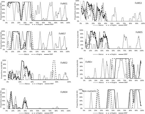
Moreover, determining measures of association requires data to be pairwise, which in this case is a problem as the total number of tasks in the three books varies considerably. However, the calculation of moving averages is not only an appropriate tool for highlighting temporal differences in the content of school mathematics textbooks (Sayers et al. 2019, Petersson et al. 2021) but also provides the starting point for calculating measures of similarity when data are not presented pairwise.

Properties of measures association in relation to smoothed data

Before we pose our research questions, there are two questions to consider. These are:

• What measures of association are suitable for comparing binary data in general and textbooks in particular?

• What happens when we smooth such data?

From the perspective of calculating measures of associatoin for binary data, the literature indicates a range of possibilities (See Cheetham and Hazel 1969, Baroni-Urbani and Buser 1976, Janson and Vegelius 1981, Romesburg 2004). Indeed, Choi, Cha and Tappert (2010) offer 76 measures of association for binary data alone. However, these measures of association tend to align with one of two main traditions, each with important implications for how one proceeds, concerning the inclusion or exclusion of simultaneous absences.

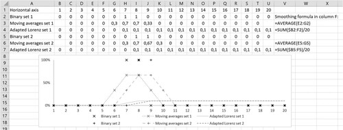
By way of illustration, rows 2 and 5 of Figure 2 show two matched sets of arbitrary data, labelled binary set 1 and binary set 2. Each is in the form of 0s and 1s denoting the absence or presence of some hypothetical object of interest. The frequencies of the coded events are identical but occur at different time points. That is, both show two cases of presence and 18 of absence. When analysing the similarity of the two sets, the first tradition, which includes simultaneous absences, shows that 90% (17 cases where both occurrences are zero and a single occurrence where both are one) are recorded as simultaneously the same. Alternatively, the second tradition, which excludes simultaneous absences, ignores the 17 pairs that are both zero and considers only the remaining three. Of these, only one pair is simultaneously the same, both being one, leading to the conclusion that the proportion of data coded as the same is 33%.

Figure 2. Data smoothing with moving averages and with adapted Lorenz-curves.

From the perspective of our analyses, particularly because all eight FoNS categories are necessary foundations for children’s learning of number (Andrews and Sayers 2015), only the first of these traditions is relevant, since any absence is as important as its presence. This holds even in the extreme case whereby both FoNS6 and FoNS8, as seen in Table 2, are absent in Singma and MNP.

However, large numbers of zero occurrences may limit the measures of association available, as division by zero would prevent the use of, for example, the Bray–Curtis distance, the Canberra distance, the Cosine coefficient and, importantly, the Pearson correlation (Romesburg 2004). However, one measure of association without this drawback is the Euclidean average distance, D, shown in Equation (1) as Euclidean similarity, being its complementary form, where the divisor N is the number of data pairs, within the compared vectors X and Y, and includes simultaneous absences. Furthermore, the Euclidean distance does not distinguish between simultaneous absences (0; 0) and simultaneous presences (1; 1) since both these have zero distance. (1) $\mathrm{Euclidean}\mathrm{similarity}=1-D=1-\sqrt{{\displaystyle \frac{1}{N}\sum {(X_j-Y_j)}^2}}$(1)

Returning to our example, the data in Figure 2 range between zero and one, and hence, the same holds for the Euclidean average distance calculated on them. Accordingly, while the Euclidean average distance D can be construed as a measure of dissimilarity, being a measure of how far one data set is from another, its complementary form, 1–D, is a measure of similarity (Romesburg 2004, 103), which, for convenience, we denote as Euclidean similarity. Euclidean similarity can be construed as an undirected measure of similarity ranging between 0 and 1, while the Pearson correlation instead is directed and ranges between –1 and 1. As an example, the Euclidean similarity in Equation (1) between the two data sets in Figure 2 is $1-\sqrt{2/20}\approx 0.68$ while their Pearson correlation instead is 0.44.

From the perspective of smoothing data, Figure 2 shows, in this particular instance, how the calculation of moving averages and adapted Lorenz-curves transform the two binary data sets into ‘continuous’ curves. One important difference between moving average curves and adapted Lorenz-curves is that while the former highlight momentary changes in the time series, adapted Lorenz-curves highlight the accumulated amount. Indeed, by definition, the construction of the adapted Lorenz-curve as a cumulative (relative) frequency makes it increase monotonically between minimum zero and maximum one unit per time step. So, for the hypothetical data in Figure 2, the Euclidean similarity between the adapted Lorenz curves is 0.98 and the Pearson correlation between them is 0.95. In particular, if the two bumps in Figure 2 were fully disjoint, the similarity of their adapted Lorenz-curves would change only little, indicating that the cumulative property of the adapted Lorenz-curves suppresses temporal differences between the data sets, hence making it unsuitable when the aim is to quantify some measure of temporal association.

By way of contrast, moving average curves preserve some of the momentary properties of the original data, though it transforms these originally mutually exclusive presences into partly overlapping curves. Hence, for the moving average curves, the Euclidean similarity becomes 0.84 and the Pearson correlation becomes 0.75. Figure 2 should make it clear that a wider moving average window further increases the overlap and consequently the value of the calculated measure of association.

This smoothing effect, due to the window width, highlights the importance of choosing a window width that corresponds to the context of the application. To illustrate what this means for educational research, we return to the textbook data shown in Table 2. The Euclidean similarities calculated on the proportions yield 0.93 between Singma and Abacus and 0.98 between Singma and MNP. Still, a visual inspection of Figure 1 indicates obvious differences in how the various learning opportunities are temporally distributed between, on the one hand, Abacus and, on the other hand, MNP and Singma.

Hence, a fine-grained temporal analysis corresponding to a narrow window may not give the same result as a coarse-grained analysis corresponding to a wide window. For example, a window of one year corresponds to the analyses undertaken by Borba and Selva (2013), Ding (2016) and Ding and Li (2010), where attention was paid only to the existence of their scrutinized topic over the course of a year. Alternatively, addressing the question, where, in the sequence of all opportunities are the learning opportunities of interest, Huntley and Terrel (2014) displayed individual occurrences of those opportunities on a timeline dot plot, corresponding to a window width of single units of analysis. A timeline dot plot allows for both visual inspection and frequency comparison of the whole textbook. However, a timeline dot plot does not allow the determination of any measure of association unless the compared textbooks have the same number of units of analysis. Thus, with research questions involving temporality and distribution, it might be relevant to exploit a window width corresponding to a week’s textbook content (Petersson et al. 2021). This, since students are likely to remember details from most of the worked through tasks during the last week’s work. Alternatively, where data stem from a transcribed lesson, the window might correspond to a range of a few minutes of classroom communication. Hence, it is important to choose a window width that is sensitive to both the research question and the context of the data.

In summary; when working with moving averages the window width should be justified by the research question in order to determine which measure of association is relevant to the research question and to avoid what might be called correlation-hacking, being analogous to the so-called p-hacking or fishing for statistical significance (Wicherts et al. 2016). A cautionary example of such correlation hacking would be the similarity calculated on the proportions in Table 2.

Finally, in this section, the various rules of thumb typically applied to correlations suggest that, say, a Pearson’s $|r|>0.7$ would be a very strong correlation, although Kozak (2009) emphasizes that such rules of thumb should be used with sensitivity to the context of the correlation. Now both Pearson’s $|r|$ and Euclidean similarity lay in the range [0; 1]. That being said, when comparing textbooks, the standard rules of thumb for weak, moderate and strong association should be applicable. A note is that the Pearson correlation ignores simultaneous absences, and hence the strength indicated by the Pearson correlation might be different from that of the Euclidean similarity, as shown in the calculated correlations for Figure 2.

Research question

As indicated above, calculating measures of association requires data to be pairwise. However, comparing two different texts remains an unsolved challenge since they typically decompose into different numbers of units of analysis. This leads to the research question for this paper: How can measures of association be calculated between non-pairwise but sequenced data? In the following, we propose two methods for addressing this problem.

Two methods for generating pairwise data

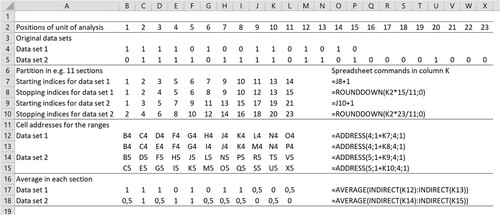
This paper applies the two methods to the large data sets in Table 2 and Figure 1, but starts with illustrating them by means of a small set of hypothetical data and standard spreadsheet tools. Figure 3 shows two hypothetical data series of which one comprises 15 data points and the other 23, where zero (0) denotes the absence of some explored characteristic and one (1) denotes its presence. Since the two sets have different numbers of data points, there are no natural matched pairs. The first method overcomes this obstacle by generating pairwise data from disjoint sections, while the second uses matching positions in overlapping sections corresponding to smoothed curves.

Figure 3. Generating pairwise data from disjoint sections.

Generating pairwise data from disjoint sections

In this first instance, we begin by splitting the two rows of data into the same number of sections, each defined by a beginning and end points that will yield single values from their arithmetic means, which will constitute the pairwise data for calculating measures of association. For the hypothetical data sets in Figure 3, column O shows the spreadsheet commands used for the calculations, while the following text explains the details. With a data set of n elements, which we wish to reduce to m sections, we create an interval of indices where the programming instruction for the k:th stopping index is $\mathrm{ROUNDDOWN}(k\cdot (n/m))$ and the starting index is $\mathrm{previous}\mathrm{stopping}\mathrm{index}+1$.

For example, in the following we show how the two data sets in Figure 3 can be reduced to pairwise data points that will allow the calculation of measures of similarity. Row 2 shows the index position for each data point of the two data sets in rows 4 and 5. Our goal is to split the two data sets into an equal number, let us say 11, of sections of equal proportions. As a calculation example, the tenth section for data set 1 starts at $\mathrm{ROUNDDOWN}(9\cdot (15/11))+1=13$ and stops at $\mathrm{ROUNDDOWN}(10\cdot (15/11))=13$ for the 10:th interval. Note that this interval starts and ends on 13. In sum, the process involves calculating all the start and stop indices, as shown in rows 7–10 of Figure 3. The only special cases are the final stopping index, which is set to 15, being the length of data set 1 and the first starting index, which is set to 1. For data set 2, a similar calculation is undertaken but with a multiplier of 23, as set 2 contains 23 data points.

Having identified the start and stop indices for each section, the next step is to calculate the mean of the two data points represented by the start index and stop index respectively. This involves two processes. First, the cell represented by each start and stop index is identified by means of the process summarized in rows 12-15. For example, for the first section of data set 1, the start data point represents the data in cell B4 and the stop data point also represents the data in cell B4. Second, as shown in rows 17 and 18, the mean is calculated to provide pairwise data for determining some measure of association. This involves the spreadsheet calculating the mean of the data found from the start to the stop cells for each section.

Though the number of sections calculated in this manner may be arbitrary, it should not be greater than the smaller of the two sets’ cardinal values, in this case 15. This ensures that each data point in the smaller data set is used exactly once. For example, were the data to be split into 20 sections, several of set 1’s data points would be used repeatedly, creating a disproportionally high impact on any calculation of similarity.

Generating pairwise data from matching positions in smoothed curves

Inspired by time series analyses, Petersson et al. (2021) highlighted the uniquely powerful contribution made by moving averages to the analysis of textbook data. In so doing, they laid the foundations for quantifying the similarity between textbooks in terms of measures of association, based on the assumption that if two sets of data are temporally similar then, irrespective of their respective cardinalities, data points at the same temporal locations would be similar. In the following, drawing on the same hypothetical data as in Figure 3, we show how smoothed curves yield pairwise data directly from the curves themselves.

The first five rows of Figure 4 are identical to those of Figure 3; row 2 shows the index positions and rows 4 and 5 gives the two data sets. To represent windows of equal time proportions, the moving averages shown in rows 7 and 8 are based on windows of width five and seven data points, which respectively is a third of the lengths of the data sets. This window width serves just as an illustration but might be too wide for practical use. In the context of this paper, this would mean an assumption that the totality of all tasks in two textbooks would cover the total content for, say, the same school year. By way of example, the formula for cell K7 would be AVERAGE(I7:M7), while that for K8 would be AVERAGE(H8:N8). Having calculated the moving averages, the aim is now to match each value in the smaller data set with the value in the larger data set that corresponds most closely to it in the temporal scheme. To this end, the figures in rows 10 and 11 show the cumulative proportion of the data points in the sequence of all data points. For example, cell K10 shows the tenth data point out of 15 for data set 1, which corresponds to $10/15\approx 67\text{\%}$. In similar vein, cell K11 shows the tenth data point out of 23 for set 2, which corresponds to $10/23\approx 43\text{\%}$.

Figure 4. Generating pairwise data from moving averages.

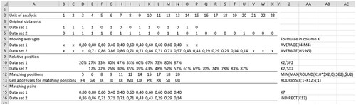
Finally, the first figure of the moving averages for data set 1, 0.80, occurs in cell D7 and corresponds to the 20% temporal point in the sequence of all data. The temporally closest value to this for data set 2 is the temporal point 22%, which corresponds to the moving average value in cell F8, being 0.86. This gives the first data pair for the calculation of a measure of similarity. A more general example can be seen in the content of cell K7, which corresponds to the 67% temporal point in data set 1’s sequence and corresponds to the 10th position in the original data and has a corresponding moving averages value of 0.60. The closest value to this in data set 2 can be seen in cell P15, which is the 65% temporal point of the data set’s sequence and corresponds to a moving average value, shown in P9, of 0.43. The spreadsheet formula for identifying the point in data set 2 that corresponds to the tenth position in data set 1 is ROUND(10/15*23). In short, Equation (2) shows the general calculation of the indices for the matching positions for two data sets of lengths short and long, where the first and last moving averages for the long data set are at positions $\mathrm{firs}{\mathrm{t}}_{\mathrm{long}}$ and $\mathrm{las}{\mathrm{t}}_{\mathrm{long}}$. (2) $\mathrm{MIN}(\mathrm{las}{\mathrm{t}}_{\mathrm{long}}\mathrm{MAX}(\mathrm{firs}{\mathrm{t}}_{\mathrm{long}}\mathrm{ROUND}((k/\mathrm{short})\cdot \mathrm{long})))$(2)

Calculating similarity from the two methods for generating pairwise data

In the following, we apply the two processes for generating pairwise data to the calculation of Euclidean similarity between the content, as represented by the various FoNS categories of competence, of the textbooks discussed earlier. In so doing, we undertake three separate sets of calculations. First, we explore the impact of different window widths on the consistency of the different similarity calculations. Second, we explore their consistency with respect to quantifying similar and dissimilar textbooks for both frequent and rare characteristics of the text. Third, we compare their consistency with respect to the Euclidean similarity with, for the sake of contrast and caution, the Pearson correlation, since these two measures of association have different properties. In so doing, we draw, when necessary, on the data for two FoNS categories, FoNS1 and FoNS 6, to illustrate our arguments when comparing, on the one hand, the two structurally similar textbooks, Singma and MNP, and, on the other hand, two different textbooks, Singma and Abacus.

Exploring the impact of different window widths on both the two pairwise calculations and Euclidean similarity

To explore the consistency of the two pairwise calculations with changing window widths, we compared the impact on Euclidean similarity of a narrow and a wide window respectively. For the former, we partition a textbook’s content into 200 sections, each approximating one school day’s workload. For the latter, we partition the same content into 40 sections each approximating one week’s workload. For the disjoint sections method and the wide window, this means splitting each data set into 40 disjoint sections while for the matching positions method, each moving average window has a width being 1/40 of the total length of each data set. The results of this process can be seen in Figure 5, comparing the Singma and Abacus, and Figure 6, comparing Singma and MNP. Both Figures 5 and 6 show that for each FoNS-category, both disjoint partitions and matching positions yield effectively identical results for each window width. In fact, for the narrow window the difference between the two methods was at most 0.01 for each FoNS-category; and for the wide window any difference was at most 0.02. Hence, both disjoint partitions and matching positions yield essentially identical measures of similarity for each window width. A detail is that the smoothing effect is more pronounced in the presence of several up and down ramps that occur at about the same temporal position in the compared textbooks.

Exploring the consistency of Euclidean similarity with similar and dissimilar textbooks

In warranting the approaches proposed in this paper, it is important to examine their sensitivity to textbook characteristics that are either rare or frequent. For example, Table 2 shows that while neither MNP nor Singma have any tasks coded for FoNS6, Abacus has six (0.5%). The Euclidean similarity between MNP and Singma is inevitably 1.0. However, as seen in Figure 5, the similarity between Abacus and Singma is 0.96 for the narrow window and 0.98 for the wide. In other words, Euclidean similarity calculations based on moving averages seem sensitive to small variations in code frequency.

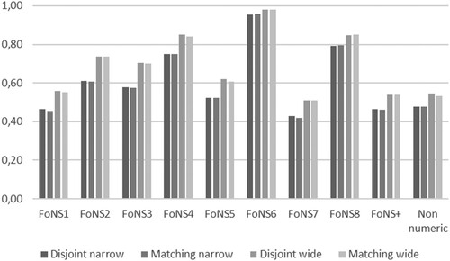
At the other extreme, Table 2 shows that around 40% of all tasks in each of the three books are coded for FoNS1. However, in both MNP and Singma, these tasks occur within the first half of the school year, while in Abacus they are distributed throughout the year. Consequently, it would be reasonable to expect measures of similarity to be sensitive to such distributive variation, with that between MNP and Singma being higher than that between Abacus and either of the other two books. This is, in fact, what can be seen in Figures 5–7. On the one hand, Figure 6 shows, with respect to FoNS1 and irrespective of window width, that the Euclidean similarity between MNP and Singma is never below 0.82. On the other hand, Figure 5 shows that the similarity between Singma and Abacus is around 0.55 for the wide window and 0.45 for the narrow, figures replicated in Figure 7, showing the similarity between MNP and Abacus. In other words, the Euclidean similarity accounts well for any distributional variation, even when the proportions of tasks found in different books are similar.

Figure 5. Euclidean similarity between Singma & Abacus.

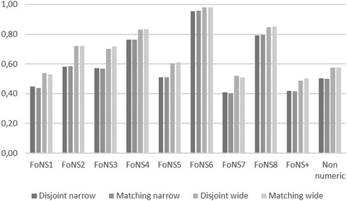
Figure 6. Euclidean similarity between Singma & MNP.

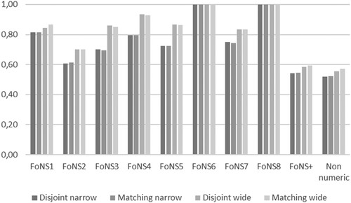
Figure 7. Euclidean similarity between Abacus & MNP.

Comparing Euclidean similarity with the Pearson correlation

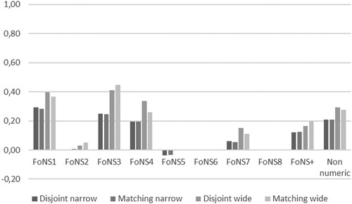
Finally, in warranting our use of Euclidean similarity, it is important to compare its outcomes with those of a conventional correlation measure. In this respect, Figure 8 offers several important insights. First, where they exist, correlations based on wide windows are typically much greater than those based on narrow windows. Second, the absence of tasks coded for FoNS6 in both Singma and MNP mean that the Pearson correlations cannot be calculated, since a division by zero necessarily results in an undefined outcome. This is in contrast with, in respect of Singma and Abacus, a Euclidean similarity of between 0.96 and 0.98 dependent on window width. Third, all the Euclidean similarities in Figure 5 indicate moderate to high correlations. In contrast, Figure 8 shows that the Pearson correlations are weak for FoNS1, FoNS3, FoNS4 and non-numeric and are negligible for other categories irrespective of the window width. In other words, where they exist, Pearson correlations tend to give a very different picture of the strength of the association between the content of textbooks, due to, as indicated earlier, their failure to account adequately for simultaneous absences. In sum, whether based on disjoint partitions or matching positions, Euclidean similarity seems to offer more robust measures of association than the Pearson correlation when simultaneous absences are common.

Figure 8. Pearson correlation between Singma & Abacus.

Conclusion

In this paper, responding to an earlier appeal for ‘new research methods’ to address a lack of correlational studies of school mathematics textbooks (Fan 2013, p. 774), we have shown how a visual and essentially qualitative interpretation of the moving averages graphs found in Petersson et al. (2021) can be augmented by a quantification of the similarity of textbooks’ content, even when they have widely differing numbers of units of analysis. In particular, we have offered two approaches to the identification of the matched-pairs necessary for calculating Euclidean similarity as a measure of association. In so doing, we have highlighted, particularly in comparison with conventional correlations, the sensitivity of Euclidean similarity to textbook features that either occur rarely or occur frequently but with widely differing temporal distributions.

Our starting point was to regard text, whether from a book, transcribed speech or action, as an ordered sequence of units of analysis. From the particular perspective of textbooks, conventional frequency analyses afford limited insights (Borba and Selva 2013, Huntley and Terrel 2014, Ding 2016); insights that can be deepened by the use of moving averages that expose the temporal distribution of the content (Sayers et al. 2019, Petersson et al. 2022). Our view is that the methods presented in this article offer additional insights in item-temporality when compared to item-frequency and item-proportionality studies on textbooks, by enabling researchers to quantify similarity of content, even when the number of data points in the compared sets are different.

To achieve this, we focused attention on three textbooks, currently used with year-one children in England and Sweden. Two of these, MNP and Singma, are translations of the same Singaporean-authored textbook, while the third, Abacus, in an English-authored text unrelated to the others. The choice of these books enabled two different but important comparisons. First, it enabled us to compare textbooks, MNP and Singma, that earlier studies had confirmed were structurally similar (Petersson et al. 2019, Sayers et al. 2019). Second, it enabled us to compare textbooks, Abacus with MNP or Abacus with Singma, known to be structurally different. Further, the use of the FoNS framework, designed to facilitate cross-cultural analyses of the opportunities afforded year-one children to acquire a core set of number competences, identified forms of learning that were commonplace in all textbooks but with differing temporal distributions, and forms of learning that were privileged in one book but absent in the others. Thus, in attending to FoNS1, number recognition, which was widely addressed in all three books, and FoNS6, estimation, which was found only in Abacus, we were able to examine how the processes outlined above played out in different circumstances.

Overall, we have shown how two methods for generating pairwise data, disjoint partitions and matching positions, yield near identical robust results when translated into a standard measure of association, in this case, Euclidean similarity. Importantly, Euclidean similarity was able to detect temporal similarities and differences between textbooks in ways that would be missed by correlations based on the same sets of pairwise data. Moreover, Euclidean similarity, due to its accounting for both simultaneous absence and presence, avoids the overinflation of correlation as a measure of association, particularly when based on, say, the relative frequencies of Table 2. This was particularly evident with respect to the Euclidean similarity calculated for FoNS1 between Abacus and, say, MNP, where tasks addressing number recognition were plentiful across all three books but distributed differently. Finally, Euclidean similarity, as shown with FoNS6, estimation, was able to account for a small presence in one book and an absence in another. This said, the present study suggests common thumb rules for assessing the strength of the association. This is due to that there is no obvious test of statistical significance of a similarity since it is not obvious to which distribution this kind of data belong. This is an area that needs further research.

As with all such approaches, whether based on disjoint partitions or matching positions it is necessary for decisions concerning window width to be determined by the research question. This is particularly important as, broadly speaking, the wider the window the higher the similarity, because wider windows smooth out local differences (see e.g. Petersson et al. 2021). In the context of this study, a research question addressing how learning opportunities are distributed throughout a lesson’s content of a textbook would demand a different window width from one focused the opportunities offered during a week.

In closing, the methods presented in this study should be applicable to forms of educational data beyond textbooks, including classroom data. One application is learning trajectories (Hunt, Westenskow et al. 2016), where individuals in two classroom settings could be compared since using the methods presented here would allow a comparison of classrooms with different numbers of lessons. Typically for this application, there are few lessons to compare, which makes it essential to have as short windows as possible. In particular, learning trajectories may have multi-level and not binary data, and may be defined to not have zero levels (1, 2, 3 etc). Hence, the Pearson correlation should work better than the Euclidean similarity since multiple levels might give the Euclidean similarity a range outside [0; 1] unless the levels are assigned as $1/n$, $2/n$, … , $n/n$. Instructional interaction patterns (Hunt and Tzur 2017), and timeline protocols (Schoenfeld 1985, Keisar and Peled 2018, Albarracin et al. 2019) are binary data just as the analysis of textbook characteristics but may differ from the latter in the following way. A task, being the unit of analysis in a textbook, typically is coded with several co-occurring codes. In contrast, if the unit of analysis for interaction patterns and timeline protocols is defined as single actions (utterances) or as very short time periods, the result may be that they in practice are mutually exclusive. A consequence of this is that there will be a lot of zeros and the temporal correlation between two classes or student groups might be similar to that of FoNS6 between two else non-similar textbooks as in Figures 5 and 7. This may be addressed by modifying the definition of the unit of analysis in order to decrease the proportion of zeros. However, research is needed for what a suitable modification might look like for this application. Finally, the authors share a data file with a calculated example in a standard spreadsheet for each of the two methods disjoint sections and matching positions. Hence there is no need for buying software licences for these two methods.

Data sharing

The authors share a data file with a calculated example for each of the two methods disjoint sections and matching positions.

Disclosure statement

No potential conflict of interest was reported by the author(s).

Additional information

Funding

The authors gratefully acknowledge the financial support of the Swedish Research Council (Vetenskapsrådet), project grant 2015-01066, without whose support the work reported in this paper would not have been possible.

References

- Alajmi, A.H., 2012. How do elementary textbooks address fractions? A review of mathematics textbooks in the USA, Japan, and Kuwait. Educational studies in mathematics, 79 (2), 239–261. doi:10.1007/s10649-011-9342-1.
- Albarracin, L., et al., 2019. Extending modelling activity diagrams as a tool to characterise mathematical modelling processes. The mathematics enthusiast, 16 (1), 211–230. https://scholarworks.umt.edu/tme/vol16/iss1/10.
- Andrews, P., and Sayers, J., 2015. Identifying opportunities for grade one children to acquire foundational number sense: developing a framework for cross cultural classroom analyses. Early childhood education journal, 43 (4), 257–267. doi:10.1007/s10643-014-0653-6.
- Baroni-Urbani, C., and Buser, M.W., 1976. Similarity of binary data. Systematic Zoology, 25 (3), 251–259.
- Borba, R., and Selva, A., 2013. Analysis of the role of the calculator in Brazilian textbooks. ZDM, 45 (5), 737–750. doi:10.1007/s11858-013-0517-3.
- Cheetham, A.H., and Hazel, J.E., 1969. Binary (presence-absence) similarity coefficients. Journal of paleontology, 43 (5), 1130–1136.
- Choi, S.-S., Cha, S.-H., and Tappert, C.C., 2010. A survey of binary similarity and distance measures. Journal of systemics, cybernetics and informatics, 8 (1), 43–48.
- Ding, M., 2016. Opportunities to learn: inverse relations in U.S. and Chinese Textbooks. Mathematical thinking and learning, 18 (1), 45–68. doi:10.1080/10986065.2016.1107819.
- Ding, M., and Li, X., 2010. A comparative analysis of the distributive property in US and Chinese Elementary Mathematics Textbooks. Cognition and instruction, 28 (2), 146–180. doi:10.1080/07370001003638553.
- Fan, L., 2013. Textbook research as Scientific Research: towards a common ground on issues and methods of research on Mathematics Textbooks. ZDM, 45 (5), 765–777. Doi: 10.1007/s11858-013-0530-6.
- Gustafsson, J.-E., and Hansen, K.Y., 2018. Changes in the impact of family education on student educational achievement in Sweden 1988–2014. Scandinavian journal of educational research, 62 (5), 719–736. doi: 10.1080/00313831.2017.1306799.
- Hunt, J., and Tzur, R., 2017. Where is difference? Processes of mathematical remediation through a constructivist lens. The journal of mathematical behavior, 48, 62–76. doi: 10.1016/j.jmathb.2017.06.007.
- Hunt, J., et al., 2016. Levels of participatory conception of fractional quantity along a purposefully sequenced series of equal sharing tasks: Stu's trajectory. The journal of mathematical behavior, 41, 45–67. doi: 10.1016/j.jmathb.2015.11.004.
- Huntley, M.A., and Terrell, M.S., 2014. One-step and multi-step linear equations: a content analysis of five textbook series. ZDM, 46 (5), 751–766. doi:10.1007/s11858-014-0627-6.
- Janson, S., and Vegelius, J., 1981. Measures of ecological association. Oecologia, 49 (3), 371–376. doi:10.1007/BF00347601.
- Jones, K., and Fujita, T., 2013. Interpretations of national curricula: the case of geometry in textbooks from England and Japan. ZDM, 45 (5), 671–683. doi: 10.1007/s11858-013-0515-5.
- Keisar, E., and Peled, I., 2018. Investigating new curricular goals: what develops when first graders solve modelling tasks? Research in mathematics education, 20 (2), 127–145. doi:10.1080/14794802.2018.1473160.
- Kozak, M., 2009. What is strong correlation? Teaching statistics, 31 (3), 85–86. doi:10.1111/j.1467-9639.2009.00387.x.
- Murray, E., McFarland-Piazza, L., and Harrison, L.J., 2015. Changing patterns of parent–teacher communication and parent involvement from preschool to school. Early child development and care, 185 (7), 1031–1052. doi: 10.1080/03004430.2014.975223.
- Petersson, J., et al., 2019. Opportunities for year-one children to acquire foundational number sense: comparing English and Swedish adaptations of the same Singapore Textbook. In: Lorraine Harbison and Aisling Twohill, eds. Proceedings of the Seventh Conference on Research in Mathematics Education in Ireland. Dublin: Institute of Education, Dublin City University, 251–258. doi:10.5281/zenodo.3580947
- Petersson, J., et al., 2021. Two novel approaches to the content analysis of school Mathematics Textbooks. International journal of research & method in education, 44 (2), 208–222. doi: 10.1080/1743727X.2020.1766437.
- Petersson, J., Sayers, J., Rosenqvist, E., and Andrews, P., 2022. Analysing English year-one mathematics textbooks through the lens of foundational number sense: A cautionary tale for importers of overseas-authored materials. Oxford Review of Education. doi: 10.1080/03054985.2022.2064443
- Romesburg, C., 2004. Cluster Analysis for Researchers. North Carolina: Lulu. com.
- Sayers, J., et al., 2019. Opportunities to learn foundational number sense in three Swedish year one textbooks: implications for the importation of overseas-authored materials. International journal of mathematical education in science and technology, 10–21. doi: 10.1080/0020739X.2019.1688406.
- Schoenfeld, A.H., 1985. Mathematical Problem Solving. Orlando: Academic Press.
- Törnroos, J., 2005. Mathematics textbooks, opportunity to learn and student achievement. Studies in educational evaluation, 31 (4), 315–327. doi: 10.1016/j.stueduc.2005.11.005.
- Wicherts, J.M., et al., 2016. Degrees of freedom in planning, running, analyzing, and reporting psychological studies: a checklist to avoid p-hacking. Frontiers in Psychology, 7, 1832. doi:10.3389/fpsyg.2016.01832.