Adaptive self-learning controllers with disturbance compensation for automatic track guidance of industrial trucks

ABSTRACT

This paper presents an extended control concept for automatic track guidance of industrial trucks in intralogistic systems. It is based on Reinforcement Learning (RL), a method of Artificial Intelligence (AI). The presented approach is able to adapt itself to different industrial truck variants and to the associated specific vehicle parameters. In order to avoid starting the whole training of the controller for each truck variant from scratch, the training process is divided into two steps. In the first step, the controller is trained on a simplified linear model using parameters of a nominal vehicle variant. Based on this, the control parameters are only fine-tuned in the second step using a more complex nonlinear model, representing the real industrial truck. In this way, the controller is adapted to the actual truck variant and the corresponding parameter values. By using the nonlinear model, it can be ensured that the forklift's dynamic is approximated within the entire operating range, even at high steering angles. Moreover, the influence of the disturbance variable of the system (path curvature) is compensated by considering this a priori knowledge within the control design. Therefore, the Artificial Neural Networks (ANN) of the RL controller and the observation vector are suitably adjusted. In this way, the occurring path curvatures can be considered in both training steps and the control parameters can be optimized accordingly. Thus, the influence of the disturbance variable can be compensated, which significantly improves the control quality. In order to demonstrate this, the new approach is compared to an RL control concept, which is not considering the disturbance variable and to a classical two-degrees-of-freedom (2DoF) control approach.

KEYWORDS:

• Artificial intelligence
• automatic control
• intelligent transportation systems
• autonomous driving
• lateral vehicle guidance
• reinforcement learning

1. Introduction

1.1. Problem description and requirements

In times of global economic markets and increasing competition, the automation of logistic processes is a basic requirement for corporate success. An important object of research and development is to increase the internal material flow via an autonomous and intelligent networked fleet, which usually consists of a wide variety of different truck variants.

An essential element in this environment is the automatic track guidance of individual industrial trucks. The main objective is to guide the truck as accurately as possible along a predefined path where only small lateral deviations occur. The classical model-based control methods with respect to automatic track guidance of a heterogeneous logistics fleet are disadvantageous for several reasons. On the one hand, these control approaches prove to be time-consuming, since the modelling of the plant and the design of the controller has to be separately carried out for each truck variant. On the other hand, the use of the extensive methods of linear control theory requires a linear model that describes the plant as accurately as possible.

However, considering the entire range of applications of forklifts, the widely used linear single-track model (Section 2) reaches its limits. This is based on the simplifying assumptions during the development process of the model. Especially the small angle approximation leads to problems with respect to industrial trucks. Due to the high demands on manoeuverability, forklifts are designed with rear-axle steering systems, allowing steering angles of up to 90${}^{\circ }$ [1]. As a result, the linear model is not able to approximate the vehicle dynamics in the entire operation mode, which can lead to significant disadvantages in the model-based design of the controller.

Since the varying path curvature during operation has a significant influence on the automatic track guidance system and the trajectory is predefined, this information represents a priori knowledge and should be exploited by control concept. Consequently, an approach has to be developed that independently adapts to different industrial truck variants, takes into account the actual dynamic of the forklift within the entire range of applications and considers existing a priori knowledge.

1.2. Related research

The papers [2–6] deal with the topic of automatic track guidance of industrial trucks, but each of them focuses only on a single truck variant.

In the publications [7–10], a 2DoF control concept for automatic track guidance of vehicles is presented, that specifically considers the influence of the disturbance variable (path curvature) as a priori knowledge. These control structures consist of a linear disturbance compensation (feedforward controller FFC) combined with different kinds of feedback controllers (FBC). These approaches proved to be very effective, since the influence of the changing path curvature can almost be compensated. Compared to a classical feedback control concept, significant advantages can be achieved using the 2DoF approach. Since both parts of the lateral controller (FFC and FBC) depend on the plant, this concept is suitable for only one single truck variant as well.

In order to consider multiple forklift variants, new methods based on AI are used in addition to the classical adaptive control concepts given in Ref. [11–13]. An overview as well as a classification of the different AI approaches is given in Ref. [14]. The well-known RL control methods suffer from the fact, that a priori knowledge is not integrated into the training process [15, 16]. Therefore, a new approach has been presented in Ref. [14] that will be called Reinforcement Learning Control Considering a priori Plant Knowledge (RLCCPK) in the following. Its basic idea consists of integrating a priori knowledge of the plant into the training, which significantly increases the efficiency of the whole process. The presented RLCCPK approach considers a priori knowledge of the controlled system but neglects the influence of the varying path curvature during operation. Since the path is available in advance, this a priori knowledge should be taken into account by the control concept. Therefore an extension of the RLCCPK approach has been presented in Ref. [17]. However, this approach uses only a simplified linear model during the training process of the RL controller, which approximates the vehicle dynamics only for a limited range of applications (Section 2.4).

1.3. Main contribution and outline of this paper

This paper presents an extended control concept for the automatic track guidance of industrial trucks which is based on RL. It adapts itself to different vehicle variants and also takes into account a priori plant knowledge. RL is implemented in the form of the so-called Twin Delayed Deep Deterministic Policy Gradient (TD3) algorithm, as it proves to be suitable for the application of automatic track guidance [18]. The method of integrating a priori plant knowledge into the training process known from RLCCPK is extended to compensate the influence of the disturbance variable and to ensure steady-state accuracy in analogy to a classical 2DoF control concept [17]. By means of an appropriate extension of the so-called observation vector the path curvature is provided to the RL controller. Furthermore, the structures of the RL controller's ANN have to be adjusted to process the information of the enlarged observation vector.

In order to guarantee a high control quality within the entire application range of the real industrial truck, the training process of the AI-based controller is divided into two steps using different plant models. In the first step, the controller is pre-trained on the basis of a simplified linear model representing a priori knowledge of the basic lateral dynamic vehicle behaviour. Since this model is derived for an industrial truck with average vehicle parameter values, a fine tuning of the control parameters with respect to the actual vehicle variant is performed in the second training step. Therefore, a more complex nonlinear model is used, representing the real industrial truck's lateral dynamic behaviour. Using this advanced model, the actual dynamics of the industrial trucks can be approximated within the entire operating range, even at high steering angles. This two-stage procedure using different plant models offers the possibility to investigate the adaptability of the already pre-trained controller to the real vehicle behaviour in simulation. In this way, both the control quality and the controller's training efficiency can significantly be improved. To demonstrate this, the control concept proposed in this paper, called Reinforcement Learning Control with Disturbance Compensation (RLCDC), is compared to the RLCCPK and a 2DoF control approach.

This paper is organized as follows. Section 2 provides the system overview and addresses both the development of the linear and nonlinear plant model and their validation using real measurement data. This section ends with the introduction of the structures of the different control approaches. In Section 3, the design of the 2DoF controller is carried out using the root locus method. The fundamentals of RL as well as the AI-based control approaches (RLCCPK and RLCDC) will be introduced in Section 4. Subsequently, the simulation results of the used control concepts are assessed (Section 5). At the end of the paper, in Section 6, the main conclusions are discussed.

2. System overview and modelling of the plant

At the beginning of this section, the principle of the automatic track guidance and the fundamental control structure are presented. Subsequently, both the linear (Section 2.2) and the nonlinear plant model (Section 2.3) are introduced. In order to illustrate the advantages of the nonlinear model, especially in the range of high steering angles, a validation of the models is presented in Section 2.4. The following Section 2.5 is dedicated to the structure of the classical 2DoF control concept, since it is used as a comparison control approach in this paper. Finally, the proposed AI-based control concept for the specific consideration of the disturbance variable (RLCDC) is presented in analogy to the 2DoF control approach in Section 2.6.

2.1. System overview

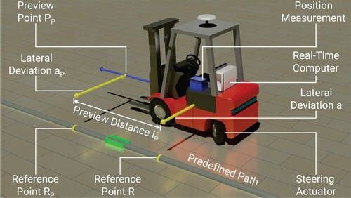
Figure 1 depicts the principle of automatic steering control of an industrial truck. First of all, the desired vehicle trajectory (predefined path) is calculated and stored as a data set on the real-time computer. The data record includes the necessary setpoint information for the automated vehicle guidance, such as the Cartesian Coordinates and curvature of the trajectory. The main objective is to guide the truck as accurately as possible along the path. In Ref. [14] it is shown, that it is of benefit to the control of the system if a preview point $P_p$ is guided instead of vehicles centre of gravity (CoG). For this purpose, $P_p$ is defined in the preview distance $l_p$ in front of the industrial truck's CoG [19]. The lateral deviation $a_p$ corresponds to the distance between the preview point $P_p$ and the reference point $R_p$ on the predefined path. Using this information, the controller calculates an appropriate control signal for the steering actuator in order to reduce the lateral deviation.

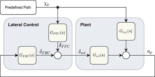
The fundamental structure of the proposed vehicle guidance system is provided in Figure 2. The plant model consists of three parts, starting with the position-controlled steering actuator. The second part is the so-called single-track model, which describes the lateral vehicle dynamics depending on the steering angle ${\delta }_r$. The last part represents the kinematics of the vehicle, i.e. its relative motion with respect to the predefined path. The curvature ${\chi }_p$ of the path in the reference point $R_p$ represents one input of the controlled system and is considered a disturbance variable. The second input is a control signal ${\delta }_{set}$ which is calculated by the lateral controller depending on the lateral deviation $a_p$, representing the output signal of the controlled system.

Figure 1. Principle of automatic track guidance.

2.2. Linear plant model

Based on the presented structure of the mathematical plant model in Figure 2, the modelling of the single parts can be given. The transmission behaviour of the position-controlled steering actuator is approximated as a first-order delay element with the delay time constant $T_s$: (1) $\dot{{\delta }_r}=-\frac{1}{T_s}\cdot {\delta }_r+\frac{1}{T_s}\cdot {\delta }_{set}$(1) The second part is the so-called single-track model [7–10, 20]. This well-known model from the literature is valid for vehicles with front-axle steering. An extension in order to describe the lateral dynamic behaviour of industrial trucks with rear-axle steering has been derived in Ref. [14]. It is obtained under the assumption that the CoG of the vehicle is at road level, which neglects the influence of wheel load distributions. Thus, the wheels of each axle can be combined into one resulting wheel. Figure 3 depicts the single track model for industrial trucks with rear-axle steering. An overview of the associated variables is given in Table 1.

Figure 2. Fundamental control structure.

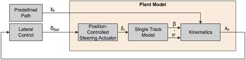
Figure 3. Single-track model with rear-axle steering.

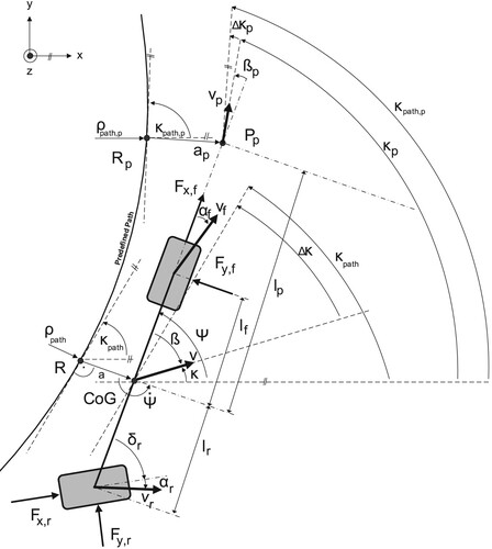
Table 1. Variables of single-track model in Figure 3.

Variables	Description
$a,a_p$	Lateral deviation, lateral deviation in $P_p$
${\rho }_{path}$	Predefined path radius
$\kappa ,{\kappa }_{path}$	Course angle, path course angle
$\mathrm{\Delta }\kappa$	Course angle deviation
$v,v_p$	Velocity CoG, velocity $P_p$
$F_f,F_r$	Tyre forces
$\text{β},{\text{β}}_p$	Side slip angle CoG, side slip angle $P_p$
$\psi ,\dot{\psi }$	Yaw angle, yaw rate
${\delta }_r$	Steer angle
${\alpha }_f,{\alpha }_r$	Front slip angle, rear slip angle
$l_f,l_r$	Distance between CoG and wheels
x, y, z	Coordinate axes

Furthermore, the following simplifying assumptions are made during the mathematical description of the lateral dynamic vehicle behaviour:

• Neglect of longitudinal dynamic forces like traction forces, braking forces and aerodynamic drag forces

• Constant or only slowly changing vehicle speed

• Small steering angles, slip angles and side slip angles

The first two assumptions can be made since the lateral vehicle dynamic motion basically changes significantly faster than the longitudinal dynamic motion. The third assumption limits the range of validity of the model. It describes the lateral vehicle dynamic behaviour only with restricted accuracy for manoeuvers with high steering angles and during the limits of driving physics. Taking into account these assumptions and adapting the linear model to forklifts with rear-axle steering, the following equations of motion are obtained: (2) $\begin{array}{rl}& m\cdot v\cdot (-\dot{\text{β}}+\dot{\psi })=F_{y,f}+F_{y,r}\end{array}$(2) (3) $\begin{array}{rl}& J_z\cdot \ddot{\psi }=F_{y,f}\cdot l_f-F_{y,r}\cdot l_r,\end{array}$(3) where m is the vehicle mass and $J_z$ is the moment of inertia at the forklifts CoG about the vertical axis. Assuming small steering angles the tyre forces $F_{y,f}$ and $F_{y,r}$ can be linearised and represented as: (4a) $\begin{array}{rl}{F}_{y,f}& =c_f\cdot {\alpha }_f\end{array}$(4a) (4b) $\begin{array}{rl}{F}_{y,r}& =c_r\cdot {\alpha }_r\end{array}$(4b) with (5a) $\begin{array}{rl}{\alpha }_f& =\text{β}-l_f\cdot \frac{\dot{\psi }}{v}\end{array}$(5a) (5b) $\begin{array}{rl}{\alpha }_r& =l_r\cdot \frac{\dot{\psi }}{v}+\text{β}-{\delta }_r\end{array}$(5b) Thus, the tyre forces are assumed to be proportional to the vehicle's slip angles ${\alpha }_f$ and ${\alpha }_r$, while the lateral tyre stiffness coefficients $c_f$ and $c_r$ are assumed to be constant.

To use the plant model for the design of the lateral controller, the model equations have to be extended to describe the relative motion of the vehicle with respect to the path (third part of the model). Specifically, the following relationship results for the lateral deviation ($a_p$) and the course angle (${\kappa }_{path}$) with respect to the preview point $P_p$ and the reference point on the predefined path $R_p$ [21, 22]. (6) $\begin{array}{rl}\mathrm{\Delta }\dot{\kappa }& ={\dot{\kappa }}_{path}+\dot{\text{β}}-\dot{\psi }\end{array}$(6) (7) $\begin{array}{rl}{\dot{a}}_p& =-l_p\cdot \dot{\psi }+v\cdot \mathrm{\Delta }\kappa \end{array}$(7) (8) $\begin{array}{rl}{\dot{\kappa }}_{path}& =\frac{v}{{\rho }_{path}}\end{array}$(8) Finally, the linear plant model can be given in state space representation Equation (9(9) $\begin{array}{rl}& \left[\begin{array}{c}\dot{\text{β}}\\ \ddot{\psi }\\ \mathrm{\Delta }\dot{\kappa }\\ {\dot{a}}_p\\ {\dot{\delta }}_r\end{array}\right]=[\begin{array}{cc}-{\displaystyle \frac{c_f+c_r}{m\cdot v}}& {\displaystyle \frac{-c_r\cdot l_r+c_f\cdot l_f}{m\cdot v^2}}+1\\ {\displaystyle \frac{-c_r\cdot l_r+c_f\cdot l_f}{J_z}}& -{\displaystyle \frac{c_r\cdot l_r^2+c_f\cdot l_f^2}{J_z\cdot v}}\\ -{\displaystyle \frac{c_f+c_r}{m\cdot v}}& {\displaystyle \frac{c_f\cdot l_f-c_r\cdot l_r}{m\cdot v^2}}\\ 0& -l_p\\ 0& 0\end{array}\\ & \begin{array}{ccc}0& 0& {\displaystyle \frac{c_r}{m\cdot v}}\\ 0& 0& {\displaystyle \frac{c_r\cdot l_r}{J_z}}\\ 0& 0& {\displaystyle \frac{c_r}{m\cdot v}}\\ v& 0& 0\\ 0& 0& -{\displaystyle \frac{1}{T_s}}\end{array}]\\ & \cdot \left[\begin{array}{c}\text{β}\\ \dot{\psi }\\ \mathrm{\Delta }\kappa \\ a_p\\ {\delta }_r\end{array}\right]+\left[\begin{array}{cc}0& 0\\ 0& 0\\ 0& v\\ 0& 0\\ {\displaystyle \frac{1}{T_s}}& 0\end{array}\right]\cdot \left[\begin{array}{c}{\delta }_{set}\\ {\chi }_p\end{array}\right]\end{array}$(9) ), where $x=[\text{β},\dot{\psi },\mathrm{\Delta }\kappa ,a_p,{\delta }_r{]}^T$ describes the state vector of the system and $u=[{\delta }_{set},{\chi }_p{]}^T$ represents the vector of its input signals. These are the steering angle setpoint, calculated by the lateral controller (control signal), as well as the curvature of the predefined path, considered as disturbance variable. Using this information and the state space model Equation (9(9) $\begin{array}{rl}& \left[\begin{array}{c}\dot{\text{β}}\\ \ddot{\psi }\\ \mathrm{\Delta }\dot{\kappa }\\ {\dot{a}}_p\\ {\dot{\delta }}_r\end{array}\right]=[\begin{array}{cc}-{\displaystyle \frac{c_f+c_r}{m\cdot v}}& {\displaystyle \frac{-c_r\cdot l_r+c_f\cdot l_f}{m\cdot v^2}}+1\\ {\displaystyle \frac{-c_r\cdot l_r+c_f\cdot l_f}{J_z}}& -{\displaystyle \frac{c_r\cdot l_r^2+c_f\cdot l_f^2}{J_z\cdot v}}\\ -{\displaystyle \frac{c_f+c_r}{m\cdot v}}& {\displaystyle \frac{c_f\cdot l_f-c_r\cdot l_r}{m\cdot v^2}}\\ 0& -l_p\\ 0& 0\end{array}\\ & \begin{array}{ccc}0& 0& {\displaystyle \frac{c_r}{m\cdot v}}\\ 0& 0& {\displaystyle \frac{c_r\cdot l_r}{J_z}}\\ 0& 0& {\displaystyle \frac{c_r}{m\cdot v}}\\ v& 0& 0\\ 0& 0& -{\displaystyle \frac{1}{T_s}}\end{array}]\\ & \cdot \left[\begin{array}{c}\text{β}\\ \dot{\psi }\\ \mathrm{\Delta }\kappa \\ a_p\\ {\delta }_r\end{array}\right]+\left[\begin{array}{cc}0& 0\\ 0& 0\\ 0& v\\ 0& 0\\ {\displaystyle \frac{1}{T_s}}& 0\end{array}\right]\cdot \left[\begin{array}{c}{\delta }_{set}\\ {\chi }_p\end{array}\right]\end{array}$(9) ) the transfer functions of the plant can be specified. The disturbance transfer function ($G_{a,\chi }\left(s\right)$) and the control transfer function ($G_{a,\delta }\left(s\right)$) are given in Equations  (10(10) $\begin{array}{rl}& G_{a,\chi }\left(s\right)=\frac{v^2}{s^2}\end{array}$(10) ) and (11(11) $\begin{array}{rl}& G_{a,\delta }\left(s\right)=K\cdot \frac{s^2+b_1\cdot s+b_0}{s^2\cdot (s+\frac{1}{T_s})\cdot (s^2+a_1\cdot s+a_0)}\end{array}$(11) ) and are used for the classical model-based control design of the 2DoF controller in Section 3. In this case, $G_{a,\chi }\left(s\right)$ describes the effects of the path curvature ${\chi }_p$ on the system's output $a_p$. $G_{a,\delta }\left(s\right)$ characterizes the dynamic behaviour of the vehicle and the steering actuator. Table 2 provides an overview of the associated values of the model parameters used in Equations  (9(9) $\begin{array}{rl}& \left[\begin{array}{c}\dot{\text{β}}\\ \ddot{\psi }\\ \mathrm{\Delta }\dot{\kappa }\\ {\dot{a}}_p\\ {\dot{\delta }}_r\end{array}\right]=[\begin{array}{cc}-{\displaystyle \frac{c_f+c_r}{m\cdot v}}& {\displaystyle \frac{-c_r\cdot l_r+c_f\cdot l_f}{m\cdot v^2}}+1\\ {\displaystyle \frac{-c_r\cdot l_r+c_f\cdot l_f}{J_z}}& -{\displaystyle \frac{c_r\cdot l_r^2+c_f\cdot l_f^2}{J_z\cdot v}}\\ -{\displaystyle \frac{c_f+c_r}{m\cdot v}}& {\displaystyle \frac{c_f\cdot l_f-c_r\cdot l_r}{m\cdot v^2}}\\ 0& -l_p\\ 0& 0\end{array}\\ & \begin{array}{ccc}0& 0& {\displaystyle \frac{c_r}{m\cdot v}}\\ 0& 0& {\displaystyle \frac{c_r\cdot l_r}{J_z}}\\ 0& 0& {\displaystyle \frac{c_r}{m\cdot v}}\\ v& 0& 0\\ 0& 0& -{\displaystyle \frac{1}{T_s}}\end{array}]\\ & \cdot \left[\begin{array}{c}\text{β}\\ \dot{\psi }\\ \mathrm{\Delta }\kappa \\ a_p\\ {\delta }_r\end{array}\right]+\left[\begin{array}{cc}0& 0\\ 0& 0\\ 0& v\\ 0& 0\\ {\displaystyle \frac{1}{T_s}}& 0\end{array}\right]\cdot \left[\begin{array}{c}{\delta }_{set}\\ {\chi }_p\end{array}\right]\end{array}$(9) )– (11(11) $\begin{array}{rl}& G_{a,\delta }\left(s\right)=K\cdot \frac{s^2+b_1\cdot s+b_0}{s^2\cdot (s+\frac{1}{T_s})\cdot (s^2+a_1\cdot s+a_0)}\end{array}$(11) ) for a nominal truck variant, the Linde E30 [1]. (9) $\begin{array}{rl}& \left[\begin{array}{c}\dot{\text{β}}\\ \ddot{\psi }\\ \mathrm{\Delta }\dot{\kappa }\\ {\dot{a}}_p\\ {\dot{\delta }}_r\end{array}\right]=[\begin{array}{cc}-{\displaystyle \frac{c_f+c_r}{m\cdot v}}& {\displaystyle \frac{-c_r\cdot l_r+c_f\cdot l_f}{m\cdot v^2}}+1\\ {\displaystyle \frac{-c_r\cdot l_r+c_f\cdot l_f}{J_z}}& -{\displaystyle \frac{c_r\cdot l_r^2+c_f\cdot l_f^2}{J_z\cdot v}}\\ -{\displaystyle \frac{c_f+c_r}{m\cdot v}}& {\displaystyle \frac{c_f\cdot l_f-c_r\cdot l_r}{m\cdot v^2}}\\ 0& -l_p\\ 0& 0\end{array}\\ & \begin{array}{ccc}0& 0& {\displaystyle \frac{c_r}{m\cdot v}}\\ 0& 0& {\displaystyle \frac{c_r\cdot l_r}{J_z}}\\ 0& 0& {\displaystyle \frac{c_r}{m\cdot v}}\\ v& 0& 0\\ 0& 0& -{\displaystyle \frac{1}{T_s}}\end{array}]\\ & \cdot \left[\begin{array}{c}\text{β}\\ \dot{\psi }\\ \mathrm{\Delta }\kappa \\ a_p\\ {\delta }_r\end{array}\right]+\left[\begin{array}{cc}0& 0\\ 0& 0\\ 0& v\\ 0& 0\\ {\displaystyle \frac{1}{T_s}}& 0\end{array}\right]\cdot \left[\begin{array}{c}{\delta }_{set}\\ {\chi }_p\end{array}\right]\end{array}$(9) (10) $\begin{array}{rl}& G_{a,\chi }\left(s\right)=\frac{v^2}{s^2}\end{array}$(10) (11) $\begin{array}{rl}& G_{a,\delta }\left(s\right)=K\cdot \frac{s^2+b_1\cdot s+b_0}{s^2\cdot (s+\frac{1}{T_s})\cdot (s^2+a_1\cdot s+a_0)}\end{array}$(11) with $\begin{array}{rl}K& =-\left(\frac{-c_r\cdot J_z+l_p\cdot c_r\cdot l_r\cdot m}{J_z\cdot m\cdot T_s}\right),\\ b_0& =\frac{c_r\cdot c_f\cdot (l_r+l_f)}{-c_r\cdot J_z+l_p\cdot c_r\cdot l_r\cdot m},\\ b_1& =\frac{c_r\cdot c_f\cdot (l_r\cdot l_f+l_f^2)-l_p\cdot c_r\cdot c_f\cdot (l_f+l_r)}{-v\cdot (-c_r\cdot J_z+l_p\cdot c_r\cdot l_r\cdot m)},\\ a_0& =\frac{c_r\cdot l_r-c_f{l}_f}{J_z}+\frac{c_r\cdot c_f\cdot (l_f+l_r{)}^2}{J_z\cdot m\cdot v^2},\\ a_1& =\frac{c_f+c_r}{m\cdot v}+\frac{c_r\cdot l_r^2+c_f\cdot l_f^2}{J_z\cdot v}\end{array}$

Table 2. Vehicle parameters of the Linde E30 [1].

Vehicle parameters	Linde E30
m	4981 kg
l	1.665 m
$c_f$	12,500 N/rad
$c_r$	50,000 N/rad
$l_f$	0.858 m
$l_r$	0.807 m
$l_p$	1.5 m
$J_z$	$3624{\mathrm{k}\mathrm{g}\mathrm{m}}^2$
$T_s$	0.2 s

2.3. Nonlinear plant model

As already mentioned, the second part of the plant model in Figure 2 describes the vehicle's dynamic. Since the rear-axle steering system of forklifts allows high steering angles, a more complex nonlinear single-track model is used [20, 23] and [24]. Compared to the linear plant model, the equations of motion are calculated to: (12) $\begin{array}{rl}& m\cdot v\cdot (-\dot{\text{β}}+\dot{\psi })=F_{y,f}\cdot \cos \text{β}+F_{y,r}\cdot \cos ({\delta }_r-\text{β})\end{array}$(12) (13) $\begin{array}{rl}& J_z\cdot \ddot{\psi }=F_{y,f}\cdot l_f-F_{y,r}\cdot l_r\cdot \cos {\delta }_r\end{array}$(13) Furthermore, the nonlinear tyre forces $F_{y,f}$ and $F_{y,r}$ are calculated using the arc-tangent approximation as described in Refs [20, 22] in dependence on the cornering stiffness coefficients $c_{f1}$,$c_{f2}$, $c_{r1}$, $c_{r2}$ as well as on the slip angles ${\alpha }_f$, ${\alpha }_r$ [10, 23, 24]. (14a) $\begin{array}{rl}{F}_{y,f}& =c_{f1}\cdot \mathrm{a}\mathrm{r}\mathrm{c}\mathrm{t}\mathrm{a}\mathrm{n}(c_{f2}\cdot {\alpha }_f)\end{array}$(14a) (14b) $\begin{array}{rl}{F}_{y,r}& =c_{r1}\cdot \mathrm{a}\mathrm{r}\mathrm{c}\mathrm{t}\mathrm{a}\mathrm{n}(c_{r2}\cdot {\alpha }_r)\end{array}$(14b) with $\begin{array}{rl}{c}_{f1}& =\frac{m\cdot g\cdot l_r}{\frac{\pi }{2}\cdot (l_f+l_r)}\cdot {\mu }_{f,max},c_{f2}=\frac{c_f}{c_{f1}},\\ c_{r1}& =\frac{m\cdot g\cdot l_f}{\frac{\pi }{2}\cdot (l_f+l_r)}\cdot {\mu }_{r,max},c_{r2}=\frac{c_f}{c_{r1}},\end{array}$${\mu }_{f,max}$ and ${\mu }_{r,max}$ correspond to the adhesion coefficients at the front and rear tyres, whereas $c_f$ and $c_r$ correspond to the cornering stiffness coefficients. With that the final equations for calculating the slip angles result in: (15a) $\begin{array}{rl}{\alpha }_f& =\mathrm{a}\mathrm{r}\mathrm{c}\mathrm{t}\mathrm{a}\mathrm{n}(\tan \text{β}-\frac{l_f}{v\cdot \cos \text{β}}\cdot \dot{\psi })\end{array}$(15a) (15b) $\begin{array}{rl}{\alpha }_r& =\mathrm{a}\mathrm{r}\mathrm{c}\mathrm{t}\mathrm{a}\mathrm{n}\left(\frac{\tan {\delta }_r-\tan \text{β}-\frac{l_r}{v\cdot \cos \text{β}}\cdot \dot{\psi }}{-1-\tan {\delta }_r\cdot \tan \text{β}-\frac{l_r\cdot \tan {\delta }_r}{v\cdot \cos \text{β}}\cdot \dot{\psi }}\right)\end{array}$(15b) Substituting the slip angles and the nonlinear tyre forces into the equations of motion, the final differential equations of the nonlinear model can be given, which are shown framed in Equations (16(16) $\boxed{{\displaystyle \begin{array}{rl}\dot{\text{β}}& =-\frac{1}{m\cdot v}\cdot [c_{f1}\cdot \mathrm{a}\mathrm{r}\mathrm{c}\mathrm{t}\mathrm{a}\mathrm{n}(c_{f2}\cdot (\phantom{\frac{l_r\cdot \tan {\delta }_r}{v\cdot \cos \text{β}}}\mathrm{a}\mathrm{r}\mathrm{c}\mathrm{t}\mathrm{a}\mathrm{n}\\ & \times (\tan \text{β}-\frac{l_f}{v\cdot \cos \text{β}}\cdot \dot{\psi })))\cdot \cos \text{β}\\ & +c_{r1}\cdot \mathrm{a}\mathrm{r}\mathrm{c}\mathrm{t}\mathrm{a}\mathrm{n}(c_{r2}\cdot (\mathrm{a}\mathrm{r}\mathrm{c}\mathrm{t}\mathrm{a}\mathrm{n}\\ & \times \left(\frac{\tan {\delta }_r-\tan \text{β}-\frac{l_r}{v\cdot \cos \text{β}}\cdot \dot{\psi }}{-1-\tan {\delta }_r\cdot \tan \text{β}-\frac{l_r\cdot \tan {\delta }_r}{v\cdot \cos \text{β}}\cdot \dot{\psi }}\right)))\\ & \cdot \cos ({\delta }_r-\text{β})\phantom{\frac{l_r\cdot \tan {\delta }_r}{v\cdot \cos \text{β}}}]+\dot{\psi }\end{array}}}$(16) )–(20(20) $\boxed{{\displaystyle \begin{array}{rl}\dot{{\delta }_r}& =-\frac{1}{T_s}\cdot {\delta }_r+\frac{1}{T_s}\cdot {\delta }_{set}\end{array}}}$(20) ):

(16) $\boxed{{\displaystyle \begin{array}{rl}\dot{\text{β}}& =-\frac{1}{m\cdot v}\cdot [c_{f1}\cdot \mathrm{a}\mathrm{r}\mathrm{c}\mathrm{t}\mathrm{a}\mathrm{n}(c_{f2}\cdot (\phantom{\frac{l_r\cdot \tan {\delta }_r}{v\cdot \cos \text{β}}}\mathrm{a}\mathrm{r}\mathrm{c}\mathrm{t}\mathrm{a}\mathrm{n}\\ & \times (\tan \text{β}-\frac{l_f}{v\cdot \cos \text{β}}\cdot \dot{\psi })))\cdot \cos \text{β}\\ & +c_{r1}\cdot \mathrm{a}\mathrm{r}\mathrm{c}\mathrm{t}\mathrm{a}\mathrm{n}(c_{r2}\cdot (\mathrm{a}\mathrm{r}\mathrm{c}\mathrm{t}\mathrm{a}\mathrm{n}\\ & \times \left(\frac{\tan {\delta }_r-\tan \text{β}-\frac{l_r}{v\cdot \cos \text{β}}\cdot \dot{\psi }}{-1-\tan {\delta }_r\cdot \tan \text{β}-\frac{l_r\cdot \tan {\delta }_r}{v\cdot \cos \text{β}}\cdot \dot{\psi }}\right)))\\ & \cdot \cos ({\delta }_r-\text{β})\phantom{\frac{l_r\cdot \tan {\delta }_r}{v\cdot \cos \text{β}}}]+\dot{\psi }\end{array}}}$(16)

(17) $\boxed{{\displaystyle \begin{array}{rl}\ddot{\psi }& =\frac{1}{J_z}\cdot [c_{f1}\cdot \mathrm{a}\mathrm{r}\mathrm{c}\mathrm{t}\mathrm{a}\mathrm{n}(c_{f2}\cdot (\phantom{\frac{l_r\cdot \tan {\delta }_r}{v\cdot \cos \text{β}}}\mathrm{a}\mathrm{r}\mathrm{c}\mathrm{t}\mathrm{a}\mathrm{n}\\ & \times (\tan \text{β}-\frac{l_f}{v\cdot \cos \text{β}}\cdot \dot{\psi })))\cdot l_f\\ & -c_{r1}\cdot \mathrm{a}\mathrm{r}\mathrm{c}\mathrm{t}\mathrm{a}\mathrm{n}(c_{r2}\cdot (\mathrm{a}\mathrm{r}\mathrm{c}\mathrm{t}\mathrm{a}\mathrm{n}\\ & \times \left(\frac{\tan {\delta }_r-\tan \text{β}-\frac{l_r}{v\cdot \cos \text{β}}\cdot \dot{\psi }}{-1-\tan {\delta }_r\cdot \tan \text{β}-\frac{l_r\cdot \tan {\delta }_r}{v\cdot \cos \text{β}}\cdot \dot{\psi }}\right)))\\ & \cdot l_r\cdot \cos {\delta }_r\phantom{\frac{l_r\cdot \tan {\delta }_r}{v\cdot \cos \text{β}}}]\end{array}}}$(17)

(18) $\boxed{{\displaystyle \begin{array}{rl}\mathrm{\Delta }\dot{\kappa }& =-\frac{1}{m\cdot v}\cdot [c_{f1}\cdot \mathrm{a}\mathrm{r}\mathrm{c}\mathrm{t}\mathrm{a}\mathrm{n}(c_{f2}\cdot (\phantom{\frac{l_r\cdot \tan {\delta }_r}{v\cdot \cos \text{β}}}\mathrm{a}\mathrm{r}\mathrm{c}\mathrm{t}\mathrm{a}\mathrm{n}\\ & \times (\tan \text{β}-\frac{l_f}{v\cdot \cos \text{β}}\cdot \dot{\psi })))\cdot \cos \text{β}\\ & +c_{r1}\cdot \mathrm{a}\mathrm{r}\mathrm{c}\mathrm{t}\mathrm{a}\mathrm{n}(c_{r2}\cdot (\mathrm{a}\mathrm{r}\mathrm{c}\mathrm{t}\mathrm{a}\mathrm{n}\\ & \times \left(\frac{\tan {\delta }_r-\tan \text{β}-\frac{l_r}{v\cdot \cos \text{β}}\cdot \dot{\psi }}{-1-\tan {\delta }_r\cdot \tan \text{β}-\frac{l_r\cdot \tan {\delta }_r}{v\cdot \cos \text{β}}\cdot \dot{\psi }}\right)))\\ & \cdot \cos ({\delta }_r-\text{β})\phantom{\frac{l_r\cdot \tan {\delta }_r}{v\cdot \cos \text{β}}}]+v\cdot {\chi }_p\end{array}}}$(18)

(19) $\boxed{{\displaystyle \begin{array}{rl}\dot{a_p}& =v\cdot \sin \mathrm{\Delta }\kappa -l_p\cdot \dot{\psi }\end{array}}}$(19)

(20) $\boxed{{\displaystyle \begin{array}{rl}\dot{{\delta }_r}& =-\frac{1}{T_s}\cdot {\delta }_r+\frac{1}{T_s}\cdot {\delta }_{set}\end{array}}}$(20)

2.4. Validation of the plant models

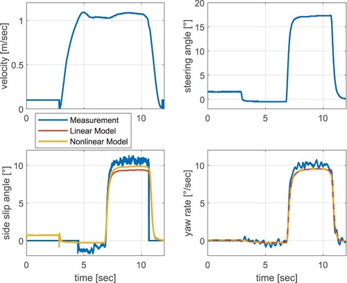
To investigate the validity of the presented single track models, three different manoeuvers are performed. For this purpose, a forklift that is comparable to the nominal Linde E30 is equipped with an Inertial Measurement Unit (IMU) and the state variables β and $\dot{\psi }$ as well as the vehicle speed v and the steering angle ${\delta }_r$ are recorded while driving. In Figure 4, the measured variables β and $\dot{\psi }$ (blue) are compared to the corresponding simulation results based on the linear (red) and nonlinear (orange) model derived above. The first manoeuver performed in the driving test deliberately involves only steering angles of up to 20${}^{\circ }$ on the rear axle. Both simulation models represent the real vehicle behaviour quite accurately and behave comparable.

If the steering angle is increased, the advantage of the nonlinear model becomes clear, which is due to the small angle approximation and the linear tyre characteristics during the development process of the linear model (Figure 5). This illustrates that the linear model is not able to approximate the lateral vehicle dynamic behaviour of industrial trucks sufficiently well within the entire operation mode, i.e. during operations with high steering angles. The nonlinear model is, therefore, able to represent the real vehicle behaviour for small as well as for higher steering angles. The fact that high steering angles actually occur during the operation of industrial trucks is demonstrated by a turning manoeuver (Figure 6). This validation illustrates again the advantage of the nonlinear model for describing vehicle dynamics of industrial trucks. Nevertheless, the linear model is quite suitable to approximate the vehicle behaviour in a limited range of operation. This a priori knowledge in the form of a validated simplified linear model will be used to pretrain the RL-controller in simulation (first step), in order to build up experience regarding the basic vehicle behaviour of a nominal forklift variant (Linde E30). Thus, based on this pre-trained RL-controller, only the fine-tuning has to be done using the more accurate and complex nonlinear model to simulate real-time operation, which significantly accelerates the training process.

Figure 4. Validation of the plant models for small steering angles.

2.5. 2DoF control structure

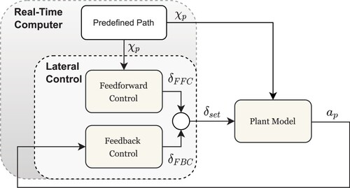
Figure 7 presents the structure of the 2DoF control concept, which can be used to compensate the influence of the disturbance variable, i.e. the path curvature [7–10, 25]. The control signal ${\delta }_{set}$ is formed by superposition of two signal components. The first part (${\delta }_{FFC}$) is calculated by an FFC that uses a priori knowledge in the form of the detailed path information, which are available in advance [21]. It determines the control signal in dependence on the path curvature ${\chi }_p$ in the current reference point $R_p$ based on the linear plant model (Section 2.2) [7].

The FBC calculates the second component (${\delta }_{FBC}$) of the control signal. Its task is to stabilize the plant and to compensating for the lateral deviation $a_p$ caused by model inaccuracies and other disturbances. In addition to the described advantages of this control concept, it has a decisive disadvantage with regard to the task of automation of a heterogeneous fleet. The FFC is not adaptive to different vehicle variants. Although the FBC can compensate for minor variances during operation, an adaptation to another truck variant is not possible with this control approach.

Figure 5. Validation of the plant models for higher steering angles.

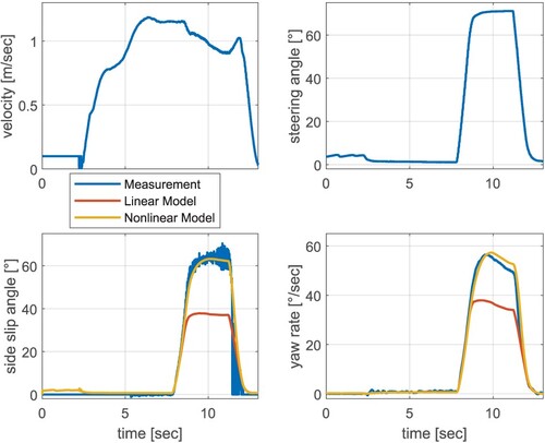
Figure 6. Validation of the plant models by a turning manoeuver.

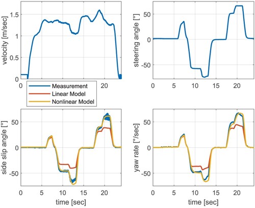
Figure 7. Structure of the 2DoF control concept.

2.6. Proposed AI-based control structure

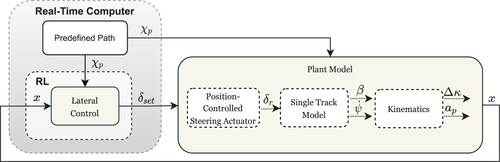
Figure 8 depicts the control structure of the proposed AI-based control concept. It is based on the RLCCPK concept given in Ref. [14]. In order to take into account the influence of the disturbance variable, the structure of the RLCCPK control concept is extended in analogy to the 2DoF concept. Since the path is defined in advance and stored on the real-time computer (Section 1), the path curvature in the reference point $R_p$ can be used as a priori knowledge. Thus, this information (${\chi }_p$) is provided to the lateral controller as an additional input signal.

The calculation of the control signal ${\delta }_{set}$ is based on the current system state x on the one hand as well as on the current path curvature in the reference point $R_p$ on the other hand. With this new control structure, the advantages of the RLCCPK and the FFC of the 2DoF control concept can be combined. It results in a new approach that is able to adapt to different vehicle variants taking into account the a priori plant knowledge and to compensate the influence of the varying path curvature during operation.

Figure 8. Structure of the proposed AI-based vehicle guidance system.

3. Design of the 2DoF controller

In Section 2, it was pointed out that the curvature of the path ${\chi }_p$ in the current reference point $R_p$ can be regarded as a disturbance variable of the lateral vehicle guidance system. Since the path is predefined and stored on the real-time computer, this a priori knowledge offers the possibility to reduce the influence of the varying path curvature during operation by means of a disturbance rejection [25]. Assuming that the mathematical model describes the controlled system accurately, the influence of the disturbance variable can completely be compensated with a suitable definition of the FFC ($G_{FFC}\left(s\right)$).

Figure 9 shows the structure of the 2DoF control concept. Its design is based on the disturbance transfer function ($G_{a,\chi }\left(s\right)$) and the control transfer function ($G_{a,\delta }\left(s\right)$) of the plant, given in Equations (10(10) $\begin{array}{rl}& G_{a,\chi }\left(s\right)=\frac{v^2}{s^2}\end{array}$(10) ) and (11(11) $\begin{array}{rl}& G_{a,\delta }\left(s\right)=K\cdot \frac{s^2+b_1\cdot s+b_0}{s^2\cdot (s+\frac{1}{T_s})\cdot (s^2+a_1\cdot s+a_0)}\end{array}$(11) ) in Section  2.2. Based on this, the following calculation of $G_{FFC}\left(s\right)$ can be derived: (21) $\begin{array}{rl}& G_{a,\chi }\left(s\right)-G_{FFC}\left(s\right)\cdot G_{a,\delta }\left(s\right)=0\\ & \Rightarrow G_{FFC}\left(s\right)=\frac{G_{a,\chi }\left(s\right)}{G_{a,\delta }\left(s\right)}\end{array}$(21) Since the resulting transfer function $G_{FFC}\left(s\right)$ (Equation (21(21) $\begin{array}{rl}& G_{a,\chi }\left(s\right)-G_{FFC}\left(s\right)\cdot G_{a,\delta }\left(s\right)=0\\ & \Rightarrow G_{FFC}\left(s\right)=\frac{G_{a,\chi }\left(s\right)}{G_{a,\delta }\left(s\right)}\end{array}$(21) )) has a higher number of zeros than poles, a first-order low-pass filter with a small time constant $T_{FFC}$ has to be added. As the FFC does not ensure a precise track guidance by itself, a FBC is used to compensate the occurring lateral deviation $a_p$. This procedure increases the robustness of the control system with respect to imprecisely known model parameters and stabilize the controlled system. The FBC is designed using the root locus method in order to achieve a damping of the dominant poles of about D = 0.7. A detailed description of the control design using root locus method has already been given in Refs [7, 9, 10]. associated transfer function ($G_{FBC}\left(s\right)$) represents the FBC as a $PD{T}_1$ controller Equation (22(22) $G_{FBC}\left(s\right)=K_{FBC}\cdot \frac{T_D\cdot s+1}{T_{FBC}\cdot s+1}$(22) ), where $K_{FBC}$ is the gain factor, $T_D$ is the derivative time and $T_{FBC}$ is the time constant of a first-order low-pass filter. The associated control parameters of the 2DoF controller are given in Table 3. (22) $G_{FBC}\left(s\right)=K_{FBC}\cdot \frac{T_D\cdot s+1}{T_{FBC}\cdot s+1}$(22)

Figure 9. Structure of the 2DoF control concept.

4. AI-based control approaches

This section is dedicated to the AI-based control approaches for the automatic track guidance of industrial trucks. At the beginning, the used methodology and the basics of RL are presented. Section 4.2 introduces the RLCCPK approach given in Ref. [14], since it is used as a comparison control concept in Section 5. Finally, the proposed RLCDC approach is discussed in Section 4.3 that specifically considers the varying path curvature during operation.

Table 3. Control parameters of the 2DoF approach.

Control parameters	Values
$T_{FFC}$	0.01 s
$K_{FBC}$	3.2634
$T_D$	0.5 s
$T_{FBC}$	0.02 s

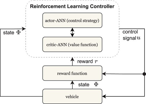
Figure 10. Principle of Reinforcement Learning.

4.1. Reinforcement learning basics

RL is a well-known approach in the domain of control systems [26–28]. It is assigned to the methods of direct neural control, since AI acts as a controller and calculates the control signal by itself. The training of the RL controller takes place in closed-loop operation and is done in analogy to the human learning process. Experiences are built up by interacting with the system. The principle of the RL process is displayed in Figure 10 and essentially consists of three blocks. The undermost block (vehicle) represents the controlled system, in this case, the industrial truck. Its current state ${\mathrm{\Phi }}_k$ is provided to the RL controller. This block describes the lateral controller that calculates the control signal $u_k$ in order to affect the controlled system. The third block (reward function) evaluates the control signal $u_k$ based on the current state ${\mathrm{\Phi }}_k$ and the following state ${\mathrm{\Phi }}_{k+1}$, in form of a feedback, called reward $r_k$. It is a measure of control quality. In analogy to the human learning process, the control strategy is adapted in order to optimize the reward.

The described basic idea of RL can be implemented using different methods. In this paper, the TD3 algorithm is used, which is an extension of the Deep Deterministic Policy Gradient (DDPG) Algorithm [27]. The TD3 algorithm is well suited for the application of automatic track guidance based on two main reasons. On the one hand, the RL controller is able to calculate a value continuous control signal which is important for a smooth vehicle track guidance. On the other hand, the training process proves to be more stable compared to the DDPG algorithm due to additional target-nets [18]. TD3 is a so-called Actor-Critic method that uses separate memory structures to differ between the control strategy $\mu \left(\mathrm{\Phi }\right)$ (actor-ANN) and the value function $Q(\mathrm{\Phi },u)$ (critic-ANN). $Q(\mathrm{\Phi },u)$ is a function to calculate the expected cumulative reward $\hat{r}$, based on its input signals Φ and u and represents the knowledge of the plant. This means, it evaluates the expected reaction of the controlled system with respect to the calculated control signal in the current system state. The optimization of the parameters ϕ of the critic-ANN is done by supervised learning, based on the obtained reward [29, 30]. The task of the actor-ANN consists of calculating the control signal $u_k$ in dependence of the current system state ${\mathrm{\Phi }}_k$ and is indicated as a function of the actor-ANN parameters θ. The optimization of this parameters (θ) should be done in order to maximize the output of the critic-ANN and thus the reward. To implement this, a criterion J is defined that describes the start distribution of $Q(\mathrm{\Phi },u)$ [27]. The basic idea is to adjust the parameters of the actor-ANN θ in the direction of the gradient ${\mathrm{\nabla }}_{\theta }J$ [18, 27, 31]. This is done by applying the chain rule with respect to the actor-ANN parameters θ (Equation (23(23) $\begin{array}{rl}{\mathrm{\nabla }}_{\theta }J& \approx \frac{1}{N}\sum _i^N{\mathrm{\nabla }}_{u}Q(\mathrm{\Phi },u|\varphi ){|}_{\mathrm{\Phi }={\mathrm{\Phi }}_i,u=\mu \left({\mathrm{\Phi }}_i\right)}\\ & \times {\mathrm{\nabla }}_{\theta }\mu \left(\mathrm{\Phi }|\theta \right){|}_{\mathrm{\Phi }={\mathrm{\Phi }}_i}\end{array}$(23) )): (23) $\begin{array}{rl}{\mathrm{\nabla }}_{\theta }J& \approx \frac{1}{N}\sum _i^N{\mathrm{\nabla }}_{u}Q(\mathrm{\Phi },u|\varphi ){|}_{\mathrm{\Phi }={\mathrm{\Phi }}_i,u=\mu \left({\mathrm{\Phi }}_i\right)}\\ & \times {\mathrm{\nabla }}_{\theta }\mu \left(\mathrm{\Phi }|\theta \right){|}_{\mathrm{\Phi }={\mathrm{\Phi }}_i}\end{array}$(23) The observation vector Φ, reflecting the state of the system, is depending on the chosen methodology. Whether the disturbance variable is taken into account (RLCDC) or not (RLCCPK), the observation vector is composed differently (Sections 4.2 and 4.3).

4.2. RLCCPK approach

The RLCCPK approach does not consider the influence of the disturbance variable (${\chi }_p$). The used observation vector Φ is formed similarly to the state vector x of the models described in Section 2 and is given in Equation  (24(24) $\mathrm{\Phi }=x=[\text{β},\dot{\psi },\mathrm{\Delta }\kappa ,a_p,{\delta }_r{]}^T$(24) ): (24) $\mathrm{\Phi }=x=[\text{β},\dot{\psi },\mathrm{\Delta }\kappa ,a_p,{\delta }_r{]}^T$(24) The behaviour of the RL controller can be specified by the definition of the reward function. The study [14] demonstrates that closed-loop behaviour of optimal state control can be approximated by choosing the reward function $r_k$ in analogy to the quadratic cost function of classical LQR [32]. In this application, the used reward function of the RLCCPK is defined to focus on minimizing the lateral deviation $a_p$ of the vehicle with respect to the path. Therefore, the weighting factor of $a_{p,k}^2$ is chosen significantly larger than the weightings of the other signals (Equation (25(25) $\begin{array}{rl}{r}_k& =-({\text{β}}_k^2+{\dot{\psi }}_k^2+\mathrm{\Delta }{\kappa }_k^2+10000\cdot a_{p,k}^2\\ & +{\delta }_{r,k}^2+5\cdot {\delta }_{set,k}^2)\end{array}$(25) )). (25) $\begin{array}{rl}{r}_k& =-({\text{β}}_k^2+{\dot{\psi }}_k^2+\mathrm{\Delta }{\kappa }_k^2+10000\cdot a_{p,k}^2\\ & +{\delta }_{r,k}^2+5\cdot {\delta }_{set,k}^2)\end{array}$(25)

4.3. Proposed RLCDC approach

In order to compensate the influence of the varying path curvature in the reference point $R_p$ during operation, the observation vector Φ of the RLCCPK (Equation (24(24) $\mathrm{\Phi }=x=[\text{β},\dot{\psi },\mathrm{\Delta }\kappa ,a_p,{\delta }_r{]}^T$(24) )) is extended by the disturbance variable ${\chi }_p$. The resulting observation vector ${\mathrm{\Phi }}_{ext}$ of the RLCDC approach is given in Equation  (26(26) ${\mathrm{\Phi }}_{ext}=\left[\begin{array}{c}\mathrm{\Phi }\\ {\chi }_p\end{array}\right]=[\text{β},\dot{\psi },\mathrm{\Delta }\kappa ,a_p,{\delta }_r,{\chi }_p{]}^T$(26) ). Thus, the current path curvature can be used for the calculation of the ideal control signal ${\delta }_{set}$ (actor-ANN). Due to the fact that ${\chi }_p$ only provides a non-zero value while driving a curve, the RLCDC approach offers the opportunity to generate an additional control signal component. In case of a control deviation caused by model inaccuracies or other disturbances, the extension of the observation (${\mathrm{\Phi }}_{ext}$) has no effect. 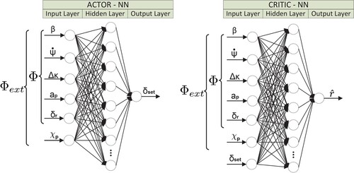(26) ${\mathrm{\Phi }}_{ext}=\left[\begin{array}{c}\mathrm{\Phi }\\ {\chi }_p\end{array}\right]=[\text{β},\dot{\psi },\mathrm{\Delta }\kappa ,a_p,{\delta }_r,{\chi }_p{]}^T$(26) Since the signals of the observation vector form the inputs of the actor-ANN and the critic-ANN of the RL controller, the structure of these networks has to be adjusted. A further neuron is integrated in the input layers of the ANN, in order to process the information of the enlarged observation vector. Figure 11 depicts a simplified representation of the structure of the actor-ANN (left) and the critic-ANN (right). In the first hidden layer of both fully connected feed-forward ANN, 400 neurons are inserted. Therefore, the extension of the input layer with additional neuron results in a large number of further ANN parameters. Since the path curvature ${\chi }_p$ is integrated into the observation vector (${\mathrm{\Phi }}_{ext}$), this information is available to both the critic-ANN and the actor-ANN.Thus, it can be used both to estimate the expected reward ($\hat{r}$) and to calculate the ideal control signal ${\delta }_{set}$. Consequently, the influence of the disturbance variable can be compensated and the control quality can be significantly improved.

In order to compare the different RL control concepts (RLCCPK and RLCDC) with each other, the reward function given in Equation  (25(25) $\begin{array}{rl}{r}_k& =-({\text{β}}_k^2+{\dot{\psi }}_k^2+\mathrm{\Delta }{\kappa }_k^2+10000\cdot a_{p,k}^2\\ & +{\delta }_{r,k}^2+5\cdot {\delta }_{set,k}^2)\end{array}$(25) ) is used for the RLCDC approach as well.

Figure 11. Simplified representation of the extended ANN structure of the RLCDC approach.

5. Control design and simulation results

In this section, the simulation results of both RL approaches (RLCCPK and RLCDC) and the 2DoF control concept are presented and compared with each other. Section 5.1 focuses on the results after the first training step of the AI-based approaches, called pre-training, that is carried out using the simplified linear plant model and the parameters of the nominal truck variant (Linde E30). The fine-tuning of the control parameters with respect to the actual dynamic behaviour of the forklift is carried out in the second training step. For this purpose, the more accurate nonlinear plant model is used, representing the real industrial truck. The simulation results of the fine-tuned AI-based controllers are presented in Section 5.2.

Finally, the adaptability of the RL concept to another vehicle variant, such as the Linde E80 will be discussed in Section 5.3. For this purpose, the second training step is performed based on the pre-trained controllers with respect to the Linde E80. Since the 2DoF control concept is not adaptive, the simulation results of the Linde E80 are also presented using the 2DoF controller designed for the nominal truck variant.

5.1. Simulation results after the first training step

This section compares the RLCCPK, RLCDC after completion of the first training step and the 2DoF controller, considering the scenario given in Figure 12 [17].

Figure 12. Test scenario I.

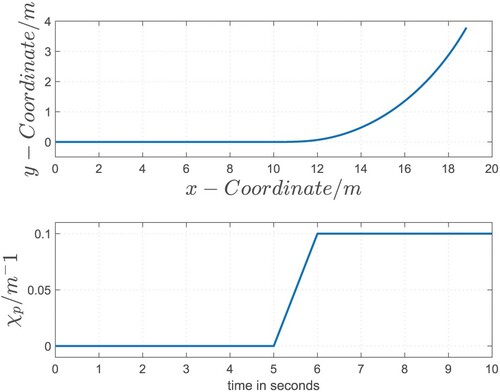
The upper part of the figure displays the course of the predefined path [ 0–20 m]. The path initially runs as a straight line [ 0–10 m] and merges into a curve with a constant curve radius ${\rho }_{path}$. The transition between the mentioned segments is realized as a clothoid [10–12 m], where the radius is linearly reduced until it reaches the final curve radius [ 12–20 m]. Since the control concepts refer to a constant velocity of v = 2m/s during the entire test scenario, the path curvature can be calculated. It is shown in the bottom part of Figure 12 and is applied to the system as a disturbance variable ${\chi }_p$ (Section 1). The industrial truck starts with an initial lateral deviation of the preview point of $a_p=0.2$m, i.e. offset from the path.

The closed-loop simulation results using the different control approaches with respect to the nominal vehicle variant (Linde E30) are presented. It shall be shown, how the different control concepts can deal with the scenario given in Figure 12 and compensate the influence of the disturbance variable. Since RLCCPK does not consider the varying path curvature during operation, this approach is trained without disturbance signals in all training epochs. In order to take into account occurring path curvatures during operation, the structure of the ANN of the RLCDC is adjusted as discussed in Section 4.3. The training process of the RLCDC controller is divided into several epochs, each of them with a different disturbance value within the range of [-0.3 $\le {\chi }_p\le$ 0.3].

Figure 13 shows the closed control loop simulation results using the linear plant model. In the upper part of the figure, the time courses of the control variable (${\delta }_{set}$) are depicted. The controlled variable ($a_p$) is illustrated below. Obviously, all three concepts are comparable in the range of [0sec – 5sec]. The lateral deviation of the RLCCPK differs from the other control concepts in the rear part [5sec – 10sec] and exhibits a permanent control deviation of about $a_p=4$ cm. This is due to the fact that the path curvature is applied to the system and not taken into account by the RLCCPK. Obviously, the extension of the RL approach (RLCDC) almost completely compensates the influence of the disturbance variable and leads to steady-state accuracy comparable to the 2DoF control approach. Based on the extension of the observation vector (${\mathrm{\Phi }}_{ext}$) with the signal of the disturbance variable (${\chi }_p$) in the current reference point $R_p$, this information is made available to the controller. Due to the additional neuron in the ANN's input layer, the path curvature can directly be incorporated into the calculation of the control signal, which leads to a significant improvement in the control quality while driving along curves. Since the used ANN are fully connected, the additional neuron within the input layer in combination with the high number of neurons of the first hidden layer, lead to a more complex ANN with a large number of additional ANN parameters. This results in a higher degree of freedom with respect to the design and improves the control quality by compensating the influence of the disturbance variable.

However, the RLCDC approach has a negative effect on the training efficiency. The additional control parameters have to be taken into account in the training process. Therefore, significant more optimization steps have to be performed. This can be seen by comparing the optimization steps carried out in the first training step of RLCCPK and RLCDC Table 4.

Figure 13. Steering angle and lateral deviation using the linear plant model (Linde E30).

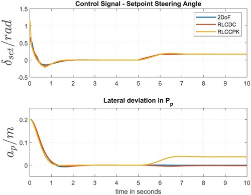
Table 4. Training efficiency of the AI-based approaches.

Control concept	Optimization steps
RLCCPK	116,822
RLCDC	295,693

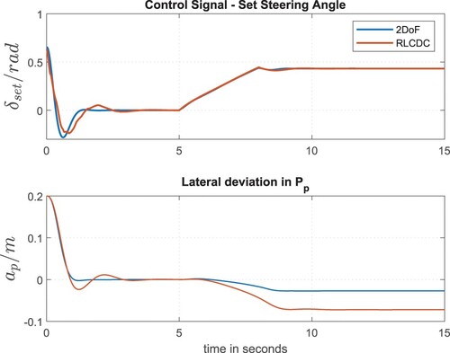
In order to ensure a safe vehicle guidance in the entire operating range of industrial trucks, the control concepts compensating the influence of the disturbance variable (RLCDC and 2DoF) are now tested on the basis of the nonlinear model. Using this model, the actual dynamic vehicle behaviour is approximated, even in applications with large steering angles. In order to get into this range, the used test scenario is changed. Therefore, a tighter curve was designed, resulting in a higher path curvature ${\chi }_p$ in the reference point $R_p$ [8 –15 s] and thus in higher steering angles during operation (Figure 14). The vehicle velocity is constant within this scenario as well (v = 2m/s).

If the controllers, designed based on the simplified linear model, are tested using the nonlinear model, the control quality suffers. Both approaches (RLCDC and 2DoF), which ensured steady-state accuracy during the simulation tests using the linear model (Figure 13) cannot guarantee it using the nonlinear one representing the real vehicle dynamics (Figure 15). In each case, a permanent control deviation occurs in the range [8 –15 s], which is about $a_p=2.8$ cm using the 2DOF and $a_p=6.4$ cm using the RLCDC.

With respect to the 2DoF controller, the fact that in case of an applied disturbance variable [8 –15 s], steady-state accuracy cannot be guaranteed is due to the FFC (Section 3), since the nonlinear plant model differs from the linear model (used for the design of the FFC). Focusing on the controlling process (2DoF) of the initial lateral deviation [0 –5 s], no significant difference can be seen compared to the investigation presented in Figure 13. Regarding to the RLCDC, the nonlinear plant model has an even stronger impact on the steady-state behaviour in case of an applied disturbance variable. It is striking that the dynamics of the closed-loop control behaviour using the RLCDC is changed in the beginning of the scenario as well. This can be explained by the fact that the control signal is not calculated exclusively on the basis of the controlled variable ($a_p$), like it is done using the 2DoF controller. Since the calculation is done by the Actor ANN, it is based on the ANN's input signals and thus on the observation vector ${\mathrm{\Phi }}_{ext}$. Due to the high steering angle in the beginning of the control process, both the side slip angle β and the yaw rate $\dot{\psi }$, as well as the other values of the observation vector, differ significantly from the values that occur during the use of the linear model. Thus, the simulation results in Figure 15 illustrate the importance of the fine-tuning step using the more accurate nonlinear plant model, which will be tested in the following section.

Figure 14. Test scenario II.

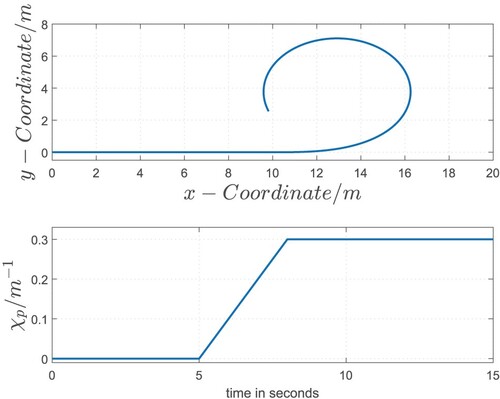
Figure 15. Steering angle and lateral deviation using the nonlinear plant model (Linde E30).

5.2. Simulation results after the second training step

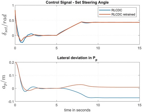
In Section 5.2, the second training step of the AI-based controller is presented, which is performed using the nonlinear plant model representing the real industrial truck. Based on the pre-trained controller (first training step) the control parameters can be adapted to the actual lateral vehicle dynamic behaviour using the nonlinear model. Figure 16 presents the simulation results of the retrained RLCDC controller (red line), using the nonlinear model and the parameters of the nominal vehicle variant. In order to illustrate the advantage of the control parameter's adaptation in the second training step, the course of the controlled variable after the first training step is also given again (blue line). Significant advantages can be achieved within the fine-tuning of the RLCDC using the nonlinear plant model. Already 2000 optimization steps (second training phase) increase the control quality and are sufficient to reduce the permanent control deviation using the RLCDC approach ($a_p=0.7$ cm) in the rear part [10–15 s] of the scenario given in Figure 14.

Figure 16. Steering angle and lateral deviation of the retrained controller using nonlinear model (Linde E30).

5.3. Investigation of the AI-based controllers adaptability

In this section, the adaption of the control concepts to another industrial truck variant is investigated. To avoid starting the entire training process from scratch, the pre-trained RLCDC of Section 5.1 is used as starting point for the second training step. The already pre-trained controller has to be adapted within the second training step (fine tuning) to the actual industrial truck variant, in this case, the Linde E80 and the associated vehicle parameters (Table 5).

Table 5. Vehicle parameters of the Linde E80 [1].

Vehicle parameters	Linde E80
m	15,720 kg
l	2.400 m
$c_f$	62,000 N/rad
$c_r$	122,000 N/rad
$l_f$	1.181 m
$l_r$	1.219 m
$l_p$	1.5 m
$J_z$	26,490 ${\mathrm{k}\mathrm{g}\mathrm{m}}^2$
$T_s$	0.2 s

By this method, the number of optimization steps can be significantly reduced compared to a training that has to be started from scratch. This can be illustrated by comparing the required optimization steps of the RCLDC in the first and second training steps given in Table 6.

Figure 17 shows the control quality of the RLCDC and 2DoF control concepts using the nonlinear plant model for the scenario II (Figure 14). It can be seen that the 2DoF controller designed for the Linde E30 is not able to stabilize the Linde E80. This is due to the fact that the model parameters and the resulting dynamics of the two vehicle variants are significantly different (Tables 2 and 5), which affects the design of both the FFC and the FBC.

The RLCDC is adapted to the changed vehicle variant and the actual industrial trucks dynamics in the second training step using the nonlinear model. After the fine-tuning process (Table 5), the re-trained RLCDC is capable of stabilizing the vehicle. The AI-based controller is still able to almost compensate the influence of the disturbance variable, which can be seen in the range of [5 –15  s] in Figure 17. A permanent control deviation of $a_p=1.6$ cm occurs. In order to be able to exactly evaluate the RLCDC's control quality, the course of the controlled variable ($a_p$) is given individually (bottom part of the figure) in addition to the comparison with the controlled variable using the 2DoF controller.

6. Conclusion

This paper presents an extension of an AI-based control approach for the automatic track guidance of industrial trucks. By separating the training process into two steps, existing a priori plant knowledge can be integrated during the training. In the first step, the controller is trained on a simplified linear model using parameters of a nominal vehicle variant. Based on this, the control parameters are only fine-tuned in the second step using a more complex nonlinear model in order to adapt to the actual vehicle variant. The use of the more complex nonlinear model represents the real industrial truck and ensures that the forklift's dynamic is approximated within the entire operating range of industrial trucks, even in operations with high steering angles. By extending the observation vector and the ANN used in the RL controller, a compensation of the influence of the path curvature is possible. Thus, the control quality of the concept can be improved and a stable control loop behaviour for different industrial truck variants can be ensured in the investigated scenarios. With the new AI-based control concept with disturbance compensation (Reinforcement Learning Control with Disturbance Compensation RLCDC), the advantages of the other presented control concepts can be combined. The adaptability with regard to new industrial truck variants of the self-learning controller presented in Ref. [14] is combined with the possibility of compensating the influence of disturbance variables of the 2DoF control concept. Finally, it should be mentioned that the RL concepts have a significant disadvantage compared to the 2DoF approach. In this configuration of the RL control approaches, all state variables of the system have to be available to the controller, whereas the 2DoF concept only requires the output variable of the plant.

Figure 17. Steering angle and lateral deviation using the nonlinear model (Linde E80).

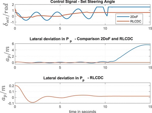
Table 6. Training efficiency of the RLCDC approach.

Control concept	Training	Optimization steps
RLCDC	1st step Linde E30	295,693
RLCDC	2nd step Linde E80	38,000

Disclosure statement

No potential conflict of interest was reported by the author(s).

Additional information

Funding

The authors gratefully acknowledge the Bavarian Ministry of Economic Affairs, Regional Development and Energy for the financial support of the project Cooperative Autonomous Intralogistic Systems under Grant No. DIK-1910-0016 and the industrial project partner: Linde Material Handling GmbH.

Notes on contributors

Timm Sauer

Timm Sauer received B.E. degree in 2016 from University of Applied Sciences Aschaffenburg, Germany, and M.S. degree in 2018 from University of Applied Sciences München, Germany. He is presently a scientific assistant in the simulation and control laboratory at University of Applied Sciences Aschaffenburg, Germany.

Manuel Gorks

Manuel Gorks received B.E. degree in 2019, M.E. degree in 2021 from University of Applied Sciences Aschaffenburg, Germany. He is presently a scientific assistant in the simulation and control laboratory at University of Applied Sciences Aschaffenburg, Germany.

Luca Spielmann

Luca Spielmann received B.E. degree in 2019, M.E. degree in 2021 from University of Applied Sciences Aschaffenburg, Germany. He is presently a scientific assistant in the simulation and control laboratory at University of Applied Sciences Aschaffenburg, Germany.

Klaus Zindler

Klaus Zindler received Dipl.-Ing. degree in 1994 from RWTH Aachen, Germany, Ph. D. degree in 1999 in control engineering from Otto-von-Guericke-Universität, Magdeburg, Germany. He was with BMW AG in Munich from 1999 to 2004, as an engineer. He is presently a professor of the Department of Engineering, Head of the simulation and control laboratory, Vice President at University of Applied Sciences Aschaffenburg and Head of Centre for Scientific Services and Transfer (ZeWiS) Obernburg, Germany.

Ulrich Jumar

Ulrich Jumar received the Dipl.-Ing. degree in 1983 and Ph. D. degree in 1986 from TH Magdeburg, Germany. He is presently a professor at the Otto-von-Guericke Universität, Magdeburg, Germany and Head of Institute of Automation and Communication Magdeburg, Germany.

References

- Linde material handling. Homepage linde material handling [updated 2022 Feb 22].
- Li L, et al. Path-following control for self-driving Forklifts based on cascade disturbance rejection with coordinates reconstruction. In: 39th Chinese Control Conference (CCC), Shenyang, China, 2020, pp. 5540–5547; 2020. doi:10.23919/CCC50068.2020.9189251.
- Tamba TA, et al. Trajectory generation of an unmanned Forklift for autonomous operation in material handling system. In: SICE AC; 2008.
- Ritzer P, et al. Advanced path following control of an overactuated robotic vehicle. In: IEEE intelligent vehicle symposium (IV); 2015.
- Bhutta MR, et al. Collision-free navigation of Forklifts by points-of-interest switching. In: international conference on URAI; 2012.
- Mohammadi A, et al. Model predictive motion control of autonomous Forklift vehicles with dynamics balance constraint. In: 14th ICCARV; 2016.
- Zindler K, et al. Querdynamische fahrzeugführung zur reproduzierbaren erprobung von sicherheitssystemen. at-Automatisierungstechnik. Oldenbourg-Verlag. 2012;60(2):61–73.
- Hahn S, et al. Two-degrees-of-freedom lateral vehicle control using nonlinear model based disturbance compensation. In: 8th IFAC-AAC; 2016.
- Heinlein S, et al. Control methods for automated testing of preventive pedestrian protection systems. Int J Veh Syst Model Test. 2015;10(2):127.
- Hahn S. Methoden zur nichtlinearen modellbasierten Spurführung benutzerdefinierter punkte an der fahrzeugfront [PhD-thesis]. 2017.
- Landau lD, et al. Adaptive control: algorithms, analysis and applications. London: Springer; 2013.
- Aström KJ, Wittenmark B. Adaptive control. 2nd ed. Reading (MA): Addison-Wesley; 1995.
- Levine W, Sawa T. The control handbook. Boca Raton, USA: CRC PRESS, IEEE Press; 1996.
- Sauer T, et al. Automatic track guidance of industrial trucks using self-learning controllers considering a priori plant knowledge. In: 5th ICCAD; 2021.
- Sallab AE, et al. End-to-End deep reinforcement learning for lane keeping assist. In: 30th conference on NIPS; 2016.
- Havenstrom ST, et al. Proportional integral derivative controller assisted reinforcement learning for path following by autonomous underwater vehicles; 2020. arXiv preprint arXiv:2002.01022.
- Sauer T, et al. Automatic track guidance of industrial trucks using AI-based controllers with disturbance compensation. In: 60th SICE annual conference; 2022.
- Fujimoto S, et al. Addressing function approximation error in actor-critic methods. In: ICML; 2018.
- Han-Shue T, et al. Developement of an automated steering vehicle based on roadway magnets – a case study of mechatronic system design. IEEE/ASME TOM. 1999;4(3):258–272.
- Pacejka H. Tyre and vehicle dynamics. 2nd ed. Oxford: Butterworth-Heinemann; 2006.
- Querregelung eines autonomen strassenfahrzeugs. Fortschr.-Ber. VDI Reihe 8, Nr. 882. VDI Verlag Düsseldorf; 2001.
- König L, et al. Nichtlineare lenkregler für den querdynamischen grenzbereich (Nonlinear steering controllers for the lateral dynamics stability limit). Automatisierungstechnik. 2007;55(6):314–321.
- König L. Ein virtueller testfahrer für den querdynamischen grenzbereich. Renningen, Germany: expert Verlag Renningen; 2009.
- Pruckner A. Nichtlineare Fahrzustandsbeobachtung und -regelung einer PKW-Hinterradlenkung. Dissertation; 2001.
- Horowitz IM. Synthesis of feedback systems. New York: Academic Press; 1963.
- Vogt M. An overview of deep learning techniques, at – automatisierungstechnik. Oldenbourg Wissenschaftsverlag. 2018;66(9):690–703.
- Lillicrap TP, et al. Continuous control with deep reinforcement learning. In: ICLR; 2016.
- Sutton R, Barto A. Reinforcement learning: an introduction. London, England: The MIT Press; 2018.
- Hagan M, et al. Neural network design. Oklahoma, USA: Martin Hagan; 2014.
- Gurney K. An introduction to neural networks. Oxford, England: UCL Press Limited; 1997.
- Silver D, et al. Deterministic policy gradient algorithms. In: ICML; 2014.
- Ichikawa Y, et al. Neural network application for direct feedback controllers. IEEE Trans Neural Netw. 1992;3(2):224–231.