Possible data-generating models of longitudinal continuous outcomes and intercurrent events to investigate estimands

Abstract

Introduction/Background

We aimed to explore data-generating models to jointly simulate outcomes and intercurrent events for randomised clinical trials to enable the investigation of estimands.

Methods

We developed four possible data-generating models for the joint distribution of longitudinal continuous clinical outcomes and intercurrent events under the scenario where they are observable: a selection model, a pattern-mixture mixed model, a shared-parameter model and a joint model of longitudinally observed outcomes and a survival model for intercurrent events. We present a case study in a short-term depression trial with repeated measurements of continuous outcomes and two types of intercurrent events, and evaluate the potential and challenges of such data-generating models.

Results

Simulating randomised trials with outcomes and intercurrent events is a complex undertaking. We found that the four possible data-generating models can simulate different types of intercurrent events and associated longitudinal outcomes. They can be used to emulate envisaged patterns of intercurrent events and outcomes informed by prior available trial data or expectations. Model and parameter choice for a given application requires further development.

Conclusion

The four possible data-generating models could be used to investigate different estimands and their properties in-depth in the design stage. Thereby they are useful tools for the selection of estimands a priori.

Keywords:

• estimand
• longitudinal outcomes, intercurrent event
• data-generating model, simulation study

Disclaimer

As a service to authors and researchers we are providing this version of an accepted manuscript (AM). Copyediting, typesetting, and review of the resulting proofs will be undertaken on this manuscript before final publication of the Version of Record (VoR). During production and pre-press, errors may be discovered which could affect the content, and all legal disclaimers that apply to the journal relate to these versions also.

Introduction

The ICH E9(R1) estimands addendum became public in December 2019, started to be adopted since, and is in the process of implementation for regulatory purposes in drug development and evaluation (1–3). It provides a structured methodological framework for the planning, conducting, and interpreting randomised clinical trials for regulatory evaluation and approval. The main aim is to add clarity and a common understanding between all healthcare stakeholders of the treatment effects targeted in clinical trials using estimands.

The estimand is defined as: “A precise description of the treatment effect reflecting the clinical question posed by the trial objective”. The estimand comprises five attributes: treatment, population, variable, population-level summary, and strategies for addressing intercurrent events (4).

Intercurrent events are defined as: “Events occurring after treatment initiation that affect either the interpretation or the existence of the measurements associated with the clinical question of interest.” The intercurrent events can therefore be of different nature and can possibly make an impact in different ways: “Examples of intercurrent events that can affect interpretation of the measurements include discontinuation of assigned treatment and use of an additional or alternative therapy. Use of an additional or alternative therapy can take multiple forms, including change to background or concomitant therapy and switching between treatments of interest. Examples of intercurrent events that would affect the existence of the measurements include terminal events such as death and leg amputation (when assessing symptoms of diabetic foot ulcers), when these events are not part of the variable itself.” Hence, the intercurrent events occurrence could require various explanatory mechanisms that may prove difficult to identify and complex to achieve through statistical modeling.

The estimands framework is still in the early stages of regulatory adoption and implementation in clinical trial conduct, (2), but triggered ample discussions in the scientific community (5-8). Healthcare stakeholders saw its potential and started to follow and apply this guidance for clinical trials to be used for regulatory purposes (5–8). There is unclarity, however, regarding which estimands are preferred in a randomised clinical trial conducted to confirm a certain claim for a therapeutic indication to be approved (9–12). There is also uncertainty around comparing statistically proposed potential estimands for a specific trial, beyond textual descriptions (which can be completely valid), whether they can be estimated and how to best estimate them. It that sense, current estimand formulations do not fully align with estimating a well-defined parameter in a statistical model. These fundamental issues could be investigated by means of simulation studies (13). To perform a proper simulation study to investigate estimands in clinical trials, we can formulate data-generating models (DGMs) to simulate outcome data and intercurrent events under clinically plausible joint mechanisms of occurrence.

There are many DGMs available that can be implemented if only the clinical outcome has to be modeled, with or without assumptions on the missing data mechanism (15,16). One of the key innovations opened with estimands is to model the association between the occurrence of intercurrent events and clinical outcomes. This association needs to appropriately enter the DGM to allow an enhanced understanding of estimands and adequate simulation. The estimand framework requires a well-defined operational and statistical approach to how intercurrent events are accounted for in the estimation of treatment efficacy in a clinical trial. Which estimand (strategy) is preferred is clearly a multidisciplinary issue following from the research question. However, the statistical and inferential properties of any estimation procedure for an estimand need to be understood within the context of an appropriate statistical model. The important challenge for most estimand strategies is that the more interesting and clinically relevant estimands assume dependence between an intercurrent event occurring and data that is not observed as a consequence of the intercurrent event or is influenced by the occurrence of the event. A similar situation occurs for data missing ‘not at random’. In that case, different underlying DGMs may be possible that introduce ‘not at random’ missingness and these correspond to different analysis models accounting for missing ‘not at random’. Inspired by this, we introduce different DGMs and modeling methods to account for the association between intercurrent events and clinical outcomes. An important finding of our research is that these cannot be uniquely fitted to the observed data either: truly different models describing the dependence between efficacy outcomes and intercurrent events may fit the observed data visually equally well. This research is intended to explore this challenge for longitudinal data in a real-life setting. Such explorations, including other simulations similar to ours (14), may support defining estimand strategies and associated modeling and estimation for future studies. In this research, we focus on four potential DGMs that can model this association between outcomes and intercurrent events.

To our knowledge, no published articles systematically investigate how to model the association between outcomes and intercurrent events (17). A search query on 3 September 2023 in PubMed of the terms {“generate”/”simulate” AND “outcomes” AND “intercurrent events”/”post-randomis/zation events”}, and screening of the very few articles suggested, resulted in zero articles that undertook this objective. We restrict this research to DGMs for randomised clinical trials in which continuous outcomes are planned to be collected longitudinally over time (repeated measurements at protocolled visits). We showcase the four possible DGMs with a short-term anti-depression trial.

Research questions:

1. What data-generating models could be used to jointly generate outcomes and intercurrent events for a generic phase III trial in simulation studies while modeling the association between them?

2. What are the complexities of this exercise?

Methods

We developed a generic case study in a short-term depression trial with repeated measurements of continuous outcomes and two types of intercurrent events, and investigate four possible DGMs to jointly generate outcomes and intercurrent events. The DGMs originate from missing data modeling and have been adapted for outcomes and intercurrent events. We describe practical considerations on how to identify and specify parameters for each possible DGM and we provide technical details on their implementation. We provide the R code used for simulations to facilitate understanding and implementation of the methods in the future.

Table

Box 1: A case study in short-term major depressive disorder trials We consider a two-arm, randomized placebo-controlled, single center, trial of six weeks duration with superiority objective. To achieve a realistic case study where we know the full data, i.e., the intercurrent events and all the outcomes before and after the intercurrent events, we fitted a longitudinal generalized least squares model to an existing dataset from a depression trial (study 003-002). We used this model to inform the final postulated model (Table 2). Based on the same depression trial, we formulated the rules for intercurrent events. The clinical outcome is Montgomery and Asberg Depression Rating Scale (MADRS10) and is planned to be measured weekly for six weeks. We simulated 500 trials (18) to allow for approximately 0.1 precision (+/-1.96*SE) in the estimate of treatment effect from the simulated trials ( supplemental material). Assumed treatment effect (δ) at end of trial at six weeks was -3.5 points on MADRS10 scale, a standard deviation (SD) of outcomes at week 6 of 7.5, to achieve 90% power (1-β) and maximum accepted type 1 error (α) of 0.025 (for a one-sided t-test) resulted in needing 95 patients per arm. We assume early separation in the outcome between the arms with the treatment effect maintained to the end of trial. Intercurrent events of interest are treatment discontinuation due to lack of efficacy (LoE) at week 3 and due to adverse events (AE) at week 2. These assumptions are based on study 003-002 (source trial for the case study). The expected proportion of LoE at trial level is 35% (21% in control, 14% in experimental)], the expected proportion of AE at trial level is 15% (5% in control, 10% in experimental). The patients not experiencing any intercurrent events are randomly allocated evenly at trial level (they are the remainder of simulated subjects that do not experience any intercurrent event). A downward time trend of outcomes is expected (improvement), based on the source trials used to extract the DGMs parameters.

The main steps for constructing the DGM are: 1) Investigate available data from completed trials (source trials), 2) postulate models corresponding to relevant clinical assumptions and extract model parameters, 3) Simulate trials with outcomes and intercurrent events, 4) Verify the generated datasets for concordance with the target trial.

In our simulations, we followed recommendations for designing and conducting simulation studies used to evaluate statistical methods for medical research (18,19).

The verification of longitudinal outcomes and intercurrent events generated with each of the four DGMs consists of two steps: verification of the longitudinal outcomes (compare numeric values of model parameters against predefined assumed true parameters and visually inspect the trajectories – no hard criterion), of the intercurrent events (compare the type, timing and percentages tabulated against predefined type, timing and percentages). Each verification is performed against the DGM-specific parameters. We evaluated the four possible data-generating models.

All simulations were conducted in RStudio (Version 1.4.1717, “Juliet Rose” (df86b69e, 2021-05-24) for macOS) with relevant packages (20–28). The verbose, annotated R script developed and used for the simulations for all four DGMs was double-checked by a researcher independent of this project. For ease of application of the four possible DGMs, we provide this R script to facilitate simulations of envisaged trials (29).

In general, the simulation typically starts from available data for outcomes and intercurrent events from already conducted trials (source trials). Models underlying the DGMs can be fitted on these data to estimate DGM’s parameters and used to simulate outcomes and intercurrent events for the target trial.

Four models (DGMs) to jointly generate outcomes and intercurrent events

The clinical setting involves $Y_{\mathrm{ij}}$ repeated measurements of continuous outcomes, the vector $Y_i$ = {$Y_{\mathrm{ij}}$}, $i=1, .,n$ patients, $j=$ visit number, with $X_i$ associated baseline covariates.

Let ${\mathrm{IE}}_{\mathrm{ij}}$ be the specific intercurrent event indicator for $Y_{\mathrm{ij}}$, with value 1 if the intercurrent event is recorded at visit j to have been experienced between visit $j-1$ and $j$ in the time interval ( $j-1,\mathrm{ j}$], and with value 0 if the intercurrent event is not experienced in the interval ( $j-1,\mathrm{ j}$], denoted by vector ${\mathrm{IE}}_i$ = {${\mathrm{IE}}_{\mathrm{ij}}$}. This means that the intercurrent event must have occurred (it is an event) before or at the latest, simultaneously when $Y_{\mathrm{ij}}$ was measured at visit $j$. This is to be closely evaluated because the intercurrent event $I{E}_{\mathrm{ij}}$ must have affected the outcome $Y_{\mathrm{ij}}$ (interpretation or existence, as per definition in E9(R1)), otherwise the intercurrent event $I{E}_{\mathrm{ij}}$ is not an intercurrent event for $Y_{\mathrm{ij}}$, but possibly for $Y_{\mathrm{ij}+1}.$

The vector $Y_i^b$ denotes the set of outcome values for patient $i$ before the intercurrent event ${\mathrm{IE}}_{\mathrm{ij}}$ is experienced, and $Y_i^a$ the set of outcome values for patient $i$ after the intercurrent event ${\mathrm{IE}}_{\mathrm{ij}}$ is experienced. $\left\{Y_{\mathrm{ij}}\right\}= {\{Y}_i^b$, $Y_i^a\}$. If $I{E}_{\mathrm{ij}}=0$_, then $Y_{\mathrm{ij}}$ is not split into $Y_{\mathrm{ij}}^{\mathrm{ab}}$ and $Y_{\mathrm{ij}}^a$.

Full data $Z_{\mathrm{ij}}$ = {$Y_{\mathrm{ij}},\mathrm{ }{\mathrm{IE}}_{\mathrm{ij}}$}, outcomes and intercurrent events, are generated based on a DGM for the simulation study.

In all four possible DGMs, there is a need of a model for the joint distribution of $Y_{\mathrm{ij}}$ and ${\mathrm{IE}}_{\mathrm{ij}}$.

High-level descriptions of the DGMs

The Selection Model (SM) conditions the occurrence of the intercurrent event on the values of the longitudinal outcomes. The Pattern-Mixture Mixed Model (PMMM) conditions the longitudinal outcomes on the intercurrent event (type, timing, etc.). The shared-parameter model (SPM) and joint model of longitudinal outcomes and survival model for intercurrent events (hereafter referred to as “JM”), do not specifically condition the outcomes directly on the intercurrent events or the intercurrent events on the outcome, but both are conditional on shared random effects.

1. Selection model (SM)

The principle of the selection model is to first generate the longitudinal outcome data ( $Y_{\mathrm{ij}}$) and then ‘select’ based on a rule which subjects experience the intercurrent events based on these outcomes, treatment, and type of intercurrent event.

Outcomes Data Generating Model for $Y_{\mathrm{ij}}$ via marginal model

From longitudinal outcomes of earlier completed studies, the trajectories parameters and variance-covariance matrix of outcomes to generate correlated residuals ${ϵ}_{\mathrm{ij}}$ (errors) can be informed. These data can be used to model the means ${(\beta }_{1j}$ and/or ${\beta }_{2\mathrm{jTreat}})$ at different visits $j$ for the longitudinal outcome trajectories (Table 1).

Other models can be used to generate the longitudinal outcome data, e.g., a model with random effects model (e.g., random intercept and/or random slope) if this describes the observed data from previous studies better.

Intercurrent events generating model (IEGM for $\mathit{IEij}$)

In the selection model approach, intercurrent events ${\mathrm{IE}}_{\mathrm{ij}}$ are only dependent on the longitudinal outcomes $Y_{\mathrm{ij}}$.

The selection model specifies the joint distribution of $Y_i$ and ${\mathrm{IE}}_i$ through models for the distribution of $Y_i$ and the conditional distribution of ${\mathrm{IE}}_i$ given $Y_i$.$$f\left(I{E}_i,Y_i|X_i,\gamma ,\varphi \right)=f_Y\left(Y_i|X_i,\gamma \right)f_{\mathrm{IE}|Y}\left(I{E}_i|X_i,Y_i,\varphi \right),$$where $\theta =(\gamma ,\mathrm{ \varphi })$, set of parameters modeling the intercurrent events ( $\varphi$) and outcomes ( $\gamma$).

The underlying assumption is that intercurrent events and their occurrence are directly connected with the clinical outcomes – either observed before or after the occurrence of the intercurrent event. Based on clinical input, for instance, if a patient does not improve by a certain difference at the end of the trial, then treatment discontinuation due to lack of efficacy is experienced at the visit mid-trial. For AEs, it could be different; if a patient does improve but insufficiently from start to mid-trial to compensate for the AE, then the patient stops treatment for AE recorded at mid-trial.

2. Pattern-mixture mixed model (PMMM)

The pattern mixture model follows a different factorisation of the joint model for $I{E}_{\mathrm{ij}}$ and $Y_{\mathrm{ij}}$. The longitudinal outcomes and the intercurrent events follow a joint distribution, through the marginal distribution of $I{E}_i$ and the conditional distribution of $Y_i$ given $I{E}_i$:

Generate the full (complete) data $Z_{\mathrm{ij}}$ = {$Y_{\mathrm{ij}},\mathrm{ }{\mathrm{IE}}_{\mathrm{ij}}$} as follows:$$f\left(I{E}_i,Y_i|X_i,\nu ,\delta \right)=f_{\mathrm{IE}}\left(I{E}_i|X_i,\delta \right)f_{Y|\mathrm{IE}}\left(Y_i|X_i,I{E}_i,\nu \right),$$ $$\left(Y_{\mathrm{ij}}|I{E}_{\mathrm{ij}}=k\right)\sim N\left(\mu \left(k\right),\Sigma \left(k\right)\right),$$where $\theta =(\nu ,\mathrm{ \delta })$, set of parameters modeling the intercurrent events ( $\delta$) and outcomes ( $\nu$).

Namely, the profiles associated with a type and timing of intercurrent event (IE) together form a pattern (in the sense of pattern mixture). The profiles in this pattern are multivariate normal distributed with a mean and covariance matrix specific to each pattern $k$.

The number of patients in each pattern can be pre-determined (specific fixed proportion of each pattern), stochastic (varying proportions of each pattern), or a mix (varying proportion of each pattern and an exact fixed proportion of certain or more patterns).

3. Shared-parameter model (SPM)

The repeated measurements ( $Y_{\mathrm{ij}}$) of continuous outcomes are modeled using a random effects model, such as a random intercept and/or random slope model (subject-specific model).

Then, the intercurrent events follow a logistic regression model (the outcome is an intercurrent event at a particular timepoint $j$) with fixed and random effects ( $b_i$). At least some of the random effects in this logistic model and some of the random effects in the model for the longitudinal outcomes are common, i.e., shared. The logistic model gives the probability for patient $i$ to experience the intercurrent event $\mathrm{IE }$ at timepoint $j$ conditional on the random effects shared with the longitudinal outcomes model, for example, a linear mixed-effects model. Each subject has latent traits expressed by random effects. Both the longitudinal outcome of the subject and the probability of experiencing an intercurrent of specific type and timing depend on this latent trait (e.g., frailty).

Outcomes sub-model

The process for repeated measurements of continuous outcomes is as follows:$$Y_{\mathrm{ij}}=X_i^Y\mathrm{*}{\beta }^Y+Z_{i\mathrm{ }}^Y\mathrm{*}{b}_i+{\epsilon }_{\mathrm{ij}},$$ $$b_i\mathrm{ }\sim \mathrm{ N}\left(0,\mathrm{ }{\sigma }_b^2\right),\mathrm{ }{\epsilon }_{\mathrm{ij}}\sim \mathrm{ N}(0,\mathrm{ }{\sigma }_{{\epsilon }_{\mathrm{ij}}}^2))\mathrm{ }.$$

${\sigma }_b^2$ is the (co)variance of the random effects

${\sigma }_{{\epsilon }_{\mathrm{ij}}}^2$ is the variance of the errors

Intercurrent events sub-model

The intercurrent events occurrence mechanism is” at random”. The intercurrent events to be experienced are conditional on random effects $b_i$, distributed as$$\mathit{logit}\left(P\left(I{E}_{\mathrm{ij}}\right)\right)=\log \hspace{0.17em}\left(\frac{P\left(I{E}_{\mathrm{ij}}\right)}{1-P\left(I{E}_{\mathrm{ij}}\right)}\right)=X_i^{\mathrm{IE}}\mathrm{*}{\beta }^{\mathrm{IE}}+Z_{i\mathrm{ }}^{\mathrm{IE}}\mathrm{*}{b}_i+{\epsilon }_{\mathrm{ij}}^{\mathit{logit}}.$$

Here $X_i^x$ is the design matrix for the fixed effects ${\beta }^x$, which could have the same/different fixed effects as used in the linear-mixed effects model to generate $Y_{\mathrm{ij}}$, or other combination of linear predictors. $Z_i^x$ is the design matrix for the random effects $b_i$. This step can require finetuning for postulated models or models can be fitted on actual data directly. Here, ${\epsilon }_{\mathrm{ij}}^{\mathit{logit}}$ represents the error term for each logit model.

For each intercurrent event, at particular timepoints $j$, a logit model can be postulated to model its occurrence based on fixed effects (e.g., covariates) and random effects.

The logit models for the estimated probabilities of occurrence of intercurrent events for specific patients at specific timepoints $j$ are directly dictated by the patients’ subject-specific random intercepts and/or slopes (shared random effects).

4. Joint modeling of repeated measurements and intercurrent events via JM

Outcomes sub-model

In the same manner as in SPM DGM (Shared-Parameter Model) (17,30,31)], the longitudinal profiles are generated via random effects as:$$Y_{\mathrm{ij}}=X_i^Y\mathrm{*}{\beta }^Y+Z_{i\mathrm{ }}^Y\mathrm{*}{b}_i+{\epsilon }_{\mathrm{ij}}=m_i^{}\left(t\right)+{\epsilon }_{\mathrm{ij}},$$ $$b_i\mathrm{ }\sim \mathrm{ N}\left(0,\mathrm{ }{\sigma }_b^2\right),\mathrm{ }{\epsilon }_{\mathrm{ij}}\sim \mathrm{ N}\left(0,\mathrm{ }{\sigma }_{{\epsilon }_{\mathrm{ij}}}^2\right)\mathrm{ }.$$

Intercurrent events sub-model

Intercurrent events are modeled with a (parametric) survival model. In our case, we use a Weibull distribution for $h_0$ to draw time to intercurrent event data for each patient:$$h_i\left(t\left|M_i^{\mathrm{*}}\right(t)\right)=h_0\left(t\right)\hspace{0.17em}\exp \hspace{0.17em}\{\gamma \mathrm{ }{\omega }_i+m_i^{\mathrm{*}}(t\left)\right\},\mathrm{ }$$ $$S_i\left(t|b_i\right)=\exp \left(-{\int }_0^t{h}_0\left(s\right)\hspace{0.17em}\exp \hspace{0.17em}\{\gamma \mathrm{ }{\omega }_i+\alpha m_i^{\mathrm{*}}(t\left)\right\}\mathrm{ds}\right),$$

Where:

$w_i$= baseline covariates

$\gamma =$ parameters for baseline covariates

$Y_i\left(t\right)=Y_{\mathrm{ij}}=\mathrm{ }$ longitudinal outcomes$$m_i^{\mathrm{*}}\left(t\right)=\left\{m_i^{\mathrm{*}}\right(s),\mathrm{ }0\le s<t\}$$

$\gamma \mathrm{*}{w}_i+{\mathrm{\alpha *m}}_i^{\mathrm{*}}\left(t\right)=$ linear predictor to generate a time to intercurrent events

$m_i^{\mathrm{*}}$= the estimated true longitudinal measurement that contains at least some or all random effects $b_i$ that are also part of the linear predictor for the outcomes $Y_{\mathrm{ij}}$;

The term ‘ $\alpha$’ is a regularisation factor that quantifies the strength of the association between the true longitudinal measurement and the risk of an intercurrent event.

The random effects contained in $m_i^{\mathrm{*}}\left(t\right)$ influence the hazard of an intercurrent event for each individual patient $i$ (subject-specific hazard). We use time as a continuous variable; if the intercurrent event falls (likely) between pre-planned visits, the next coming visit in time can be considered to have recorded the intercurrent event. Other survival models could be used for $h_0$, for instance, a discrete hazard function (time as a categorical variable) is also 'concrete' enough to generate a survival curve (and related quantities).

Trial design features and setup for simulations

The following trial design features need to be set: type of outcome, number and timing of visits, number of trial arms, randomisation ratio, assumed trajectories of patients’ outcomes (DGM model parameters) and objective of the study, the expected outcome over time without treatment (natural history) or under control treatment and after stopping investigational treatment, and how they relate with the intercurrent events and the mechanism of occurrence, as well as relevant covariates.

While planning the simulation, the following trial design considerations can be followed to decide the settings of trial design features and which of the four possible DGMs is suited to use: type, timing (e.g., at specific timepoints or spread throughout the trial duration, early, late, uniformly or non-uniformly distributed throughout the trial), percentages at the trial level, within the arm and the ratios between them at trial and arm level, and how they relate with the outcomes, the dependency on outcomes.

Results

We present findings and describe the thought process from this comprehensive exercise tasked to better understand the interplay of outcomes and intercurrent events, to impactfully use the estimands framework.

For the case study described below, we simulated the targeted short-term major depressive disorder trial with outcomes and intercurrent events using all four possible DGMs to model the association between outcomes and intercurrent events.

We described for each DGM the considerations for implementation in Appendix 1.

Description of the target trial parameters for the four models

1. Selection Model

We display SM DGM with the deterministic rule implementation. The corresponding graphs and table for SM DGM stochastic implementation are in the supplemental material (Appendix 4).

Please see Table 1 for the interpretation of these parameters.

For treatment discontinuation due to lack of efficacy, we apply the same rule for both arms based on the within-patient difference at visit 6 ( $D_{i6}=Y_{i0}-Y_{i6}$). If $D_{i6}$ < 5 points on MADRS10 (insufficient efficacy), then treatment discontinuation due to lack of efficacy will be assigned at $j=3$ for that particular patient.

For treatment discontinuation due to adverse event, we apply a different rule for each arm based on observed efficacy and the assumed relation between very high efficacy and the occurrence of AE.

The intercurrent event IE is assumed to occur between day 8 and day 14 inclusively and recorded at the day 14 visit (see described above in the Selection Model DGM). $D_{i1}=Y_{i0}-Y_{i1}$.

For the experimental arm, if $D_{i1}$ > 3, then treatment discontinuation due to adverse event at $j=2$ for that particular patient. This corresponds to a steep decrease in MADRS10 observing good (or too much) efficacy, but the patient experiences AE due to toxicity or accumulation additional to the perceived efficacy.

For the control arm, if $D_{i1}\mathrm{ }\le$ -2, then treatment discontinuation due to adverse events at $j=2$ for that particular patient; as for control arm patients there is likely no relation between high efficacy and AE. This corresponds possibly to a non-decrease in MADRS10 to some extent; if the patient experiences AE and insufficient efficacy, the benefit to AE-detrimental effect ratio is not positive to stay in the trial, AE being the main reason. To steer the percentages of treatment discontinuations due to adverse event, all control patients that meet this deterministic rule have subsequently a probability $P_{A{E}_{\mathit{Treat}}}$ to experience the AE. $P_{A{E}_{\mathit{Treat}}}$ is sampled for each simulated trial from a uniform distribution with mean $\mathit{proportio}{n}_{\mathrm{AE}}$ to add more variability. This range of the uniform distribution is chosen such that the ratios for LoE:AE within arms are within the parameters mentioned above.

For the deterministic implementation of the SM DGM, these probabilities have to be set in accordance with the rules for intercurrent events (as possibly observed in actual trials) and with the desired percentages of intercurrent events to be achieved. The rules for intercurrent events limit the maximum percentages of each intercurrent event that can be simulated (e.g., how many patients in the trial have a decrease from baseline of less than 5 points on the MADRS10 scale).

For the stochastic implementation, the percentages depend on the linear predictor terms. Below are model parameters that were fitted on a very large trial where the profiles and intercurrent events were simulated based on the above SM DGM deterministic implementation. Subsequently, these models will follow stochastically the rules for intercurrent events and corresponding percentages.

${\mathit{\varphi }}_0=\mathit{intercept}, {\mathit{\varphi }}_1=$ parameter for the outcome difference of interest according to the rules for intercurrent events.

Unless the rules for LoE and AE exclude each other, there may be competing events in the SMs. In that case, the earlier event (the AE) takes priority and will be assigned.

2. Pattern-Mixture Mixed Model

The order of operations for the PMMM DGM is to identify the patterns (i.e., the subsets of patients with a given type and timing of intercurrent event) and estimate the longitudinal parameters for each pattern. In concordance with the proportions of each pattern at the trial level and concordance with the overall trial parameters, the weighting of these patterns must be refined, such that the weighted averages correspond when stacking (see weighted average formula below) together the patterns and comprising the (full) target trial.$$\mathit{weighted average for treatment effect at week j}=$$ $$\frac{{\sum }_{p=1}^m{\beta }_{{\mathit{pattern}}_p^{\mathit{control}}}^j{\text{ * }W}_{{\mathit{pattern}}_p^{\mathit{control}}}}{{\sum }_{p=1}^m{W}_{{\mathit{pattern}}_p^{\mathit{control}}}}\frac{{\sum }_{p=1}^m{\beta }_{{\mathit{pattern}}_p^{\exp }\mathrm{ }}^j\mathrm{* }{W}_{{\mathit{pattern}}_p^{\exp }}\mathrm{ }}{{\sum }_{p=1}^m{W}_{{\mathit{pattern}}_p^{\exp }}}$$

$$w_p=\mathit{weight or proportion of a pattern of intercurrent events in a certain arm}$$

$m=\mathrm{a certain pattern of intercurrent events or behaviour}$ (“AE”, “LoE” or “No intercurrent events”, respectively)

$$\exp =\mathit{experimental arm}$$

3. Shared-Parameter Model

Below are the estimated, refined and used parameters for the linear mixed-effects and logistics regression models used to simulate trials with the SPM DGM.

$\mathit{logit}\left(P\left({\mathit{LoE}}_{\mathrm{ij}}\right)\right)={(\beta }_0+b_{i1}\mathrm{*\alpha })+\mathrm{ }{c}_1\mathrm{*Trea}{t}_i$, $\mathit{logit}\left(P\left(A{E}_{\mathrm{ij}}^{\mathit{Treat}}\right)\right)={\beta }_0+b_{i1}\mathrm{*\alpha }$, $\mathit{logit}\left(P\left(A{E}_{\mathrm{ij}}^{\mathit{Control}}\right)\right)={\beta }_0+b_{i1}$, $b_{i1}=\mathit{random slopes}$ (the same as in the linear-mixed effects model for the continuous outcomes).

For each patient, a random intercept and slope are drawn. Together with the fixed effects, these generate the longitudinal profile and the probability of experiencing an intercurrent event. Thus, the intercurrent event data are generated by drawing from a Bernoulli distribution with mean $p=$ individual probability to experience the intercurrent event $I{E}_{\mathrm{ij}}$ according to Table 6.($$I{E}_{\mathrm{ij}}|\mathrm{ }{b}_{\mathrm{ix}}\mathrm{ }\sim \mathit{Bernoulli}(P\left({\mathrm{IE}}_{\mathrm{ij}}\right))$$( $$\mathrm{Lo}{E}_{i3}|\mathrm{ }{b}_{i1}\mathrm{ }\sim \mathit{Bernoulli}(P\left({\mathit{LoE}}_{i3}\right))$$

The treatment discontinuation due to LoE to be experienced by patient $i$ at timepoint $j=3$ is Bernoulli distributed with mean equal to the probability of patient $\mathrm{i }$ to experience LoE at timepoint 3. This probability of each patient $\mathrm{i }$ is given by the logit models, including the individual random effects (shared with the longitudinal outcomes model).

Depending on the random effects variances, their distribution and symmetry relative to the position on the sigmoid logit curve, and their weight in the linear predictor of the logit models for intercurrent events, the obtained percentages of intercurrent events may vary. We conducted checks with small weights in the linear predictor and obtained precisely the percentages we desired. Another finetune to be made is an adjustment in the model such that the percentage of LoE is as desired and due to the competition with AE. Hence, an adjustment can be made, approximately, to obtain the expected percentages of LoE. Precise percentages can be achieved by decreasing variance of random effects, decreasing their weight in the linear predictor, or y increasing the number of patients and/or simulated trials.

4. Joint Model

Below are the parameters estimated, refined and used for linear predictors in the survival models for intercurrent events used to simulate trials with the SPM DGM. The linear mixed-effects model parameters are the same as those used in the SPM DGM.

Survival model parameters$$\mathit{linear predictor lack of efficacy }\left(L{P}_{\mathit{LoE}}\right)={({\beta }_0+\mathrm{ b}}_{i0}\mathrm{*\alpha })+c_1\mathrm{*Treat},$$ $$\mathit{time to lack of efficacy}={\left(-\frac{\log \hspace{0.17em}\left(U\right)}{\mathrm{\lambda }\mathrm{ exp}\left\{L{P}_{\mathit{LoE}}\right\}}\right)}^{1/\nu }$$ $$\mathit{linear predictor adverse events}\left(L{P}_{\mathrm{AE }}\right)={({\beta }_0+\mathrm{ b}}_{i0}\mathrm{*\alpha })+c_2\mathit{*Treat},$$ $$\mathit{time to adverse events }={\left(-\frac{\log \hspace{0.17em}\left(U\right)}{\mathrm{\lambda }\mathrm{ exp}\left\{L{P}_{\mathrm{AE}}\right\}}\right)}^{1/\nu }$$

To inform the model specification, joint models can be fitted on the source trial data (e.g., Weibull model for survival data as described above) (32). These models can be then used directly to simulate the intercurrent events data. Another implementation for the survival models would be an iterative process to finetune the model parameters (scale, shape) such that the distribution of intercurrent event times is the one envisaged. In particular, patients with no intercurrent event have their event time beyond the trial duration.

Intercurrent events are here generated (drawn from the Weibull distribution), such that most of the treatment discontinuations due to lack of efficacy are experienced at weeks two and three, the rest of the proportions distributed through the entire trial duration. The percentage of patients steers percentages of intercurrent events with their event time beyond the trial duration.

All model parameters for each pattern (each intercurrent event) in the DGMs have been informed by models fitted on actual trial data. In different disease settings or case studies, other parametric or semi-parametric Cox survival models could be used.

Inspection of outcomes and intercurrent events for the four DGMs

For the visual inspection of outcomes and intercurrent events, the last simulated trial (from the set of $n=$500 simulated with each DGM) was selected. The clinical outcomes were graphed and inspected to check the longitudinal trajectories for each pattern (treatment discontinuation due to lack of efficacy, treatment discontinuation due to adverse event, no intercurrent events). A spaghetti plot is provided for an actual depression trial [(33)] that visualises the longitudinal outcomes (MADRS10) of patients. This is used as an anchor to real-life trial data (not simulated), figure 1. These simulated trials are displayed by pattern and at the trial level for the patterns generated by each DGM (Figure 2 treatment discontinuation due to lack of efficacy, Figure 3 treatment discontinuation due to adverse event, Figure 4 no intercurrent event)), Figure 5 all patterns stacked together).

0= control (placebo), 1= treatment (mirtazapine)

To verify the intercurrent events percentages and prespecified ratios within the trial and between arms, we summarise the percentages of intercurrent events by type and timing (Tables 8 a-d).

Tables 8 a-d. Percentages of intercurrent events for each DGM (a = SM, b = PMMM, c = SPM and d = JM)

Comparison of the DGMs

All four DGMs that model the association of the longitudinal outcomes and intercurrent events can be informed by already conducted trials.

The only DGM that can ensure exact numbers and constant percentages of intercurrent events across all simulated trials is PMMM. The other three DGMs can ensure approximately the desired percentages of intercurrent events but still need subtle finetuning to do so. Each DGM could simulate multiple intercurrent events, possibly at different timings, for an individual patient.

The longitudinal profiles of the SM and PMMM DGMs are more flexible than SPM and JM. The SPM and JM put restrictions due to the specification and covariance of random effects and the change in group means. This is not present in the SM and PMMM DGMs because of their marginal specification of group means at each visit and unstructured residuals covariance matrix. Consequently, the random effect for intercept and slope determines the group means (and correlations) (34).

Upon visual inspection, we observed the types of trajectories and intercurrent events characteristics as envisaged to be generated, with varying degrees of precision. Acceptability of the variations of precision will depend on the purpose of the simulation.

Any of the four DGMs may be used with different modeling methods, e.g., the PMMM may be used with linear mixed effects models for repeated measures-(MMRM) generated patterns instead of the marginal model. The probabilities of intercurrent events may also depend on baseline covariates and outcome data. Each of these DGMs may be combined with elements from the other DGMs. For instance, the JM may be combined with a selection rule on the slopes to define trajectories of an intercurrent event more precisely (steep slope leading to AE, positive slope leading to LoE). The $\alpha$ regularisation (association) factor had small values in the JM, but the random effects may be given larger weights in the linear predictor of the survival model to create a stronger association.

All models needed subtle finetuning to establish and preserve the ratios of intercurrent events at the trial level. One may need to prioritise AEs over LoE occurring for the same patient (AE earlier). This can be done while obtaining the desired final percentages of LoE, after adjusting for AE first/priority because they are observed at week 2 earlier than LoE observed at week 3.

Discussion

With this research, we developed four possible DGMs to model the association between outcomes and intercurrent events, illustrated by a target trial in depression. All four DGMs can successfully simulate the target trials with varying degrees of precision. All were deemed acceptable, with the desired longitudinal trajectories and desired types, timings, and percentages of intercurrent events. The SM, SPM and JM are more suited to qualitative replication of the target trial, while PMMM can simulate it with high precision and fidelity.

The E9(R1) Addendum did not explicitly specify or suggest any kind of relationship between intercurrent events and outcomes measured before or after the intercurrent event occurrence and the SM, PMMM and SPM/JM implement each different kind of associations. These four DGMs cannot cover all possible models for associations that could exist. With a bird's eye view, all four DGMs could replicate the trial (intercurrent events and outcomes data) reasonably well. This is against the background that a choice between models can fundamentally not be made based on available observations alone. This is conceptually alike the fact that ‘missing-at-random’ cannot be tested to distinguish from a ‘missing-not-at random’ mechanism.

The SM DGM simulates intercurrent events conditional on outcomes. Rules can be formulated to describe how intercurrent events depend on the longitudinal outcomes. It can be implemented using deterministic rules or stochastic models, both implementations equally successful in simulating intercurrent events. This DGM has an intuitive understanding for treatment discontinuation due to lack of efficacy intercurrent event; for instance, if a patient is not recording sufficient efficacy by or at a certain visit, then the patient will experience treatment discontinuation due to lack of efficacy. It is possibly the simplest DGM to use from a computational perspective if there are more qualitative and open requirements on the joint distribution of longitudinal data and intercurrent events. In contrast, to reproduce a quite specified target trial may require exploring a range of rules.

The PMMM DGM simulates outcomes conditional on (patterns of) intercurrent events. Namely, the trajectories of patients will depend on the pattern of intercurrent events they belong to. This DGM also has an intuitive understanding; the patients having a specific type of intercurrent event at a specific timing will likely have some similarity in longitudinal trajectories. It is a difficult DGM to use from a computational perspective. Given data of a source trial, it requires sufficient intercurrent events in each pattern to estimate the longitudinal models of each pattern. This way, it can simulate trials with high accuracy and fidelity to the source trial.

The SPM DGM simulates outcomes and intercurrent events for a patient given her/his associated random effects. Each patient has a propensity to experience an intercurrent event conditional on random effects from the model for longitudinal outcomes (not on the actual outcomes as SM DGM). As the shared random effect models an association, this also holds the other way around: the trajectory before the intercurrent event depends on the intercurrent event via the random effects. The parameters could be estimated from fitting the SPM to the source data, if available. It is also complex to use, from a computational perspective, but can simulate intercurrent events in the desired percentages.

The JM DGM also simulates outcomes and intercurrent events that are associated through the shared random effects, but distinctly from the SPM, the generation of intercurrent events is via random effects in the linear predictor of the survival model instead of a logistic model. Also here parameters could be estimated from fitting the model to source data. It can simulate intercurrent events (with timings) distributed throughout the trial and this makes it attractive from a clinical plausibility perspective.

The DGMs are functions that can generate outcomes (and intercurrent events) corresponding to a certain treatment effect defined by (a function of) some of the parameters of the DGM. For SM this parameter is ${\beta }_{2\mathrm{JTreat}}$, for PMMM it is the weighted average for the treatment effect (a function of some of the parameters), and for SPM and JM it is ${\beta }_2$, all at the end of the trial (after 6 weeks of treatment), corresponding to the treatment effect at this visit. This corresponds to the estimand definition in the sense of Lehmann & Casella ((35)).The four possible DGMs can be used for different objectives. The SM, SPM and JM are less precise DGMs when compared to PMMM, but they are still qualitatively capable of simulating a target trial. If the objective is to have a qualitatively replicated trial, where the aim is to simulate specific patterns of intercurrent events, but without the need to obtain a specific percentage of intercurrent events at trial level, then the SM, SPM and JM are suited. If the objective is to have a precisely replicated trial, where the aim is to simulate specific patterns of intercurrent events, with the need to obtain a specific percentage of intercurrent events at specific timepoints within each arm, then the PMMM is suited.

Depending on the objective of the simulation, other (trial) characteristics may be needed.

For the illustration of the case study, the objective of the simulation was to replicate qualitatively the target trial.

For successful and meaningful use of these four possible DGMs in simulating trial data with outcomes and intercurrent events, the estimands addendum framework should be used in conjunction. Hence, a multidisciplinary approach is strongly encouraged, and multiple stakeholders should be engaged in the interaction to simulate trial data (outcomes and intercurrent events) appropriately. The SM DGM needs and allows the most clinical input for the selection rules to be realistic and plausible, as should be with estimands. The PMMM DGM only needs longitudinal data for each pattern and requires minimal or no finetuning. We found that more work may be needed in the SPM and JM, as refinement may be needed for the logistic or survival model to achieve the expected frequency (and timing) in the intercurrent events.

The different DGMs differ in their capabilities.

Firstly, we observed in the simulations that the SPM and JM DGMs encounter more difficulty in capturing the different profiles associated with different intercurrent events than the SM and PMMM DGMs). There is no separation between the longitudinal patterns for the different intercurrent events. They are more mixed together than the ones in SM and PMMM DGMs (See Figures 2-5). Intuitively, this can be understood as follows. Firstly, the shared random effects approach generates longitudinal profiles in the same class (e.g., linear). Secondly, the random effects capture only deviations from the overall mean profile, so the logistic/survival submodels can only select ‘bands’ of profiles to experience an intercurrent event. Here ‘bands’ (similar intercept and slope) are random effects’ values that in the linear predictor are mapped to the same range. In an actual trial, at least to some extent, one would expect to observe a sort of separation between patterns. For instance, one could expect LoE under a “not at random mechanism”, but it is simulated using a shared parameter model with a linear-mixed effects model, thus under an “at random” mechanism.

A distinct capability of the PMMM is that the model parameters for treatment effect in each pattern can be refined such that the weighted average of treatment effect at each visit is always as prespecified at the (targeted) trial level (See tables 2 and 4).

Furthermore, the SM and PMMM can easily be used to generate other group trajectories than the one used in the case study (34). If there is a late separation of the treatment effects or an early separation of group trajectories but no treatment effect at the end of trial, then these two DGMs could be better/more straightforward to use than the SPM or JM.

Another difference between the DGMs is that in SPM and JM, the intercurrent events can only be associated with observed outcomes and follow, in this sense, can only follow an “at random” mechanism. “Not at random” mechanisms can only be used with the SM and PMMM DGMs, and the SM can actually use both (depending on whether the selection rule is based on observed or also not observed data).

When looking at the number of intercurrent events per patient, the PMMM is the only DGM that can generate exactly one intercurrent event per patient without the competition of multiple intercurrent events on the same patient. This is possible due to the nature of PMMM, namely, one pattern is described by one (or more) intercurrent event(s). Unlike the other DGMs, based on a selection rule or on shared random effects, one patient could experience intercurrent events coming from different rules or models. Separate handling for these situations would therefore be implemented in close consideration to the rules for intercurrent events (SM) or of the shared random effects (SPM and JM).

The choice between the four possible DGMs cannot be decided solely on the source data because the DGMs depend on unobserved characteristics of the models and because the source trial data are incomplete. Hence, clinical considerations are important and needed to decide which DGM should be used for simulation studies.

Limitations:

We did not evaluate quantitatively how successful the four possible DGMs were in simulating datasets mirroring the source trial. We relied primarily on visual inspection. We did not define a quantitative criterion.

We did not consider the problem of modeling and simulating intercurrent events and missing data (in the sense of E9(R1), i.e., not following an intercurrent event). We highlight some questions that we did not aim to answer in this research: what if missing data are considered MAR, e.g., depending on outcomes observed up to the missing data, but those outcomes themselves are affected by intercurrent events that are depending on future (unobserved) outcomes (under a “not at random mechanism” such as the SM DGM)? How can this be appropriately modeled?

More research is needed to investigate such questions, and the possible implications in other settings or designs beyond the current and specific use of the four possible DGMs described.

Our four possible DGMs can have various applications.

More than one DGM could be used to generate a target trial. This could be a possible way to verify the robustness of assumptions for that target trial (e.g., at the planning and design stages). For instance, sample size estimation in relation to the constructed estimand for the primary objective. Also, DGMs could be used for the evaluation of estimation methods, sample size considerations integrating estimands, alignment of data collection with the targeted estimand, evaluation of multiple estimands of interest that could be estimated from the same trial and other areas such as estimands in adaptive trials, estimands for meta-analysis or estimands in rare disease settings. It could also be the (undiscussed) case that an estimand could be changed based on the simulation results, should they indicate so. Although, it may be debatable whether the targeted estimand should really be changed if the simulations show that the estimation of the estimands may be difficult.

As a final remark, we showed how the four DGMs work based on actual depression trials (source trials). However, these possible DGMs can be transported to other types of designs, outcomes, intercurrent events, etc., as the idea remains the same.

Conclusion

The four possible data-generating models could be used to investigate different estimands and their properties in-depth in the design stage. Thereby they are useful tools for the selection of estimands a priori.

Acknowledgements

We thank Rutger van den Bor, PhD, for double-checking the accuracy and correctness of the R code developed and used for these simulations.

Authors’ note

The views expressed in this article are the personal views of the author(s) and may not be understood or quoted as being made on behalf of or reflecting the position of the regulatory agency/agencies or organisations with which the author(s) is/are employed/affiliated.

Supplementary materials

Code

The R script (verbose) is available for all four DGMs on GitHub at https://github.com/TheMarianMitroiuTest, under a CC-BY-4.0 License.

Table 1. Outcomes DGM specification and notation (Selection Model)

$Y_{\mathrm{ij}}=({\beta }_{1j}+{\epsilon }_{\mathrm{ij}})+{\beta }_{2\mathrm{jTreat}}\mathrm{*Treatmen}{t}_i$

$Y_{\mathrm{ij}}$ = repeated measurements of continuous outcome for patient $i$ at baseline (j = 0) or follow-up visit $j$ $(e.g.,\mathrm{ j}=1,\dots , 6)$ ${\epsilon }_{\mathrm{ij}}\sim \hspace{0.25em}N(0,{\Sigma }_{{\epsilon }_{\mathrm{ij}}}^2)$ $\mathit{Trea}{t}_i$ = randomised treatment for patient $i$, indicator is 0 for control and 1 for treatment ${\epsilon }_{\mathrm{ij}}$= correlated residuals for patient $i$ at baseline (0) and follow-up visit $j$ (week 1 to week 6) ${\Sigma }_{{\epsilon }_{\mathrm{ij}}}^2$= unstructured covariance matrix of residuals ${\epsilon }_{\mathrm{ij}}$

Table 2. Assumed true parameters for trajectories in each arm for the target trial

Parameter name	Parameter value
beta.baseline ( ${\beta }_{10}$)	29.79
beta_week1 ( ${\beta }_{11}$)	−1
beta_week2 ( ${\beta }_{12}$)	−1.5
beta_week3 ( ${\beta }_{13}$)	−2
beta_week4 ( ${\beta }_{14}$)	−2.5
beta_week5 ( ${\beta }_{15}$)	−3
beta_week6 ( ${\beta }_{16}$)	−3.5
beta_v1_treatment ( ${\beta }_{21\mathrm{Treat}}$)	−1
beta_v2_treatment ( ${\beta }_{22\mathrm{Treat}}$)	−1.5
beta_v3_treatment ( ${\beta }_{23\mathrm{Treat}}$)	−2
beta_v4_treatment ( ${\beta }_{24\mathrm{Treat}}$)	−2.5
beta_v5_treatment ( ${\beta }_{25\mathrm{Treat}}$)	−3
beta_v6_treatment ( ${\beta }_{26\mathrm{Treat}}$)	−3.5

Table 3. Parameters extracted and used for linear predictors in the logit models for intercurrent events for the SM DGM, stochastic implementation

Logistic regression model	Parameter name	Parameter value
LoE at trial level	${\varphi }_0^{\mathrm{Lo}{E}_{\mathit{trial}}}$	1.077405
	${\varphi }_1^{\mathrm{Lo}{E}_{\mathit{trial}}}$	−0.355617
AE in experimental arm	${\varphi }_0^{A{E}_{\exp }}$	−2.370965
	${\varphi }_1^{A{E}_{\exp }}$	0.272188
AE in control arm	${\varphi }_0^{A{E}_{\mathit{ctrl}}}$	−2.78108
	${\varphi }_1^{A{E}_{\mathit{ctrl}}}$	−0.39944

Table 4. Model parameters for each pattern of the PMMM DGM

Parameters	Proportions:	0.35	0.15	0.50	Check at parameter level
	Trial level	LoE in both arms	AE in both arms	No IE in both arms
		0.14 in exp 0.21 in ctrl	0.10 in exp 0.05 in ctrl	1:1 random unconstrained
Betas	29.79	29.79	29.79	29.79	29.79
Beta1	−1	1	0.1	-2.75	−1.01
Beta2	−1.5	1.2	0.1	-3.85	−1.49
Beta3	−2	1.2	0.1	-4.85	−1.99
Beta4	−2.5	1.8	0.3	-6.35	−2.5
Beta5	−3	2.8	1	-8.25	−2.995
Beta6	−3.5	0	0	-7	−3.5
Beta7	−1	0.1	-2	-0.7	−1.006756703
Beta8	−1.5	0.8	-4	-1.15	−1.508520608
Beta9	−2	-0.2	-4	-1.5	−1.992814326
Beta10	−2.5	-0.5	-3.4	-2.25	−2.504744698
Beta11	−3	-0.5	-5	-2	−2.986739496
Beta12	−3.5	-1	-5	-4	−3.486994798

Table 5. Model parameters for SPM DGM

Linear mixed-effects model

Parameter name	Parameter value
Fixed effects
${\beta }_0$	29.374914
${\beta }_1$	−0.529752
${\beta }_2$	−0.577650
Random effects
$b_i\sim \mathrm{ N}(0, {\sigma }_b^2)$	${\sigma }_b^2=\left(\begin{array}{cc}21.140783& 1.307053\\ \mathrm{ }1.307053& 1.044141\end{array}\right)$
Random error
${\epsilon }_i \sim \mathrm{ N}(0, {\sigma }_i^2 )$	$\sigma = 3.285955\mathrm{ }$

Table 6. Model parameters for logit models of SPM DGM

Logistic regression model	Parameter name	Parameter value
LoE at trial level	${\beta }_0$	−0.0877193
	$c_1$	−0.60629
	$\alpha$	1
AE in experimental arm	${\beta }_0$	−1.353383
	$\alpha$	1
AE in control arm	${\beta }_0$	−2.155388
	$\alpha$	1

Table 7. Parameters of the survival models for intercurrent events in the JM DGM

Survival model	Parameter name	Parameter value
LoE at trial level	${\beta }_0$	$2.8789$
	$c_1$	$0.3111$
	$\alpha$	$-0.0279$
	$\lambda$	$1.7618$
	$\nu$	$1.7618$
AE at trial level	${\beta }_0$	$3.7550$
	$c_2$	$-0.5394$
	$\alpha$	$0.0076$
	$\lambda$	$0.9719$
	$\nu$	$0.9719$

Table 8a. Descriptive statistics intercurrent events

Selection Model DGM – deterministic rule

	Control		Treatment		Total
Intercurrent event	N	%	N	%	N	%
AE	10.1	5.3	18.1	9.5	28.2	14.9
LoE	39.5	20.8	26.8	14.1	66.3	34.9
Total	49.6	26.1	44.9	23.6	94.5	49.8

Averaged over 500 simulated trials. Trial sample size = 190

Table 8b. Descriptive statistics intercurrent events

Pattern-mixture mixed model DGM

	Control		Treatment		Total
Intercurrent event	N	%	N	%	N	%
AE	10	5.3	19	10.0	29	15.3
LoE	40	21.1	27	14.2	67	35.3
Total	50	26.4	46	24.2	96	50.6

Averaged over 500 simulated trials. Trial sample size = 190

Table 8c. Descriptive statistics intercurrent events

Shared parameter model DGM

	Control		Treatment		Total
Intercurrent event	N	%	N	%	N	%
AE	9.9	5.2	19.7	10.4	29.6	15.6
LoE	40.8	21.5	25.6	13.5	66.4	34.9
Total	50.7	26.7	45.3	23.9	96.0	50.5

Averaged over 500 simulated trials. Trial sample size = 190

Table 8d. Descriptive statistics intercurrent events

Joint model DGM

	Control		Treatment		Total
Intercurrent event	N	%	N	%	N	%
AE	10.0	5.2	19.3	10.1	29.2	15.4
LoE	41.7	21.9	24.6	12.9	66.2	34.9
Total	51.7	27.1	43.9	23.0	95.4	50.3

Averaged over 500 simulated trials. Trial sample size = 190

Figure 1. Individual trajectories by treatment arm/study 003-021

Graphs to visualise each pattern in the trials simulated with each DGM

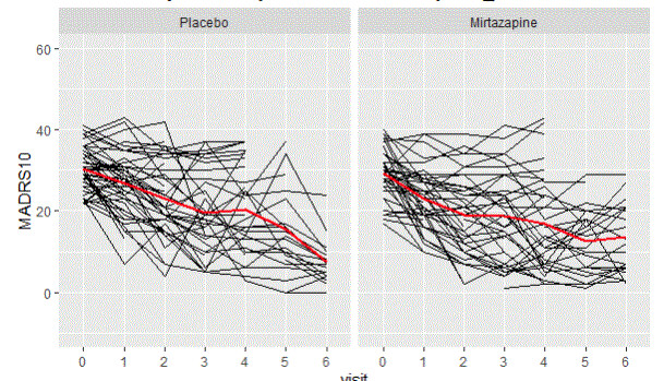
Figure 2. Treatment discontinuation due to lack of efficacy patterns by each DGM and arm

Figure 3. Treatment discontinuation due to adverse event patterns by each DGM and arm

Figure 4. No intercurrent events patterns by each DGM and arm

Figure 5. All patterns stacked together as a trial simulated by each DGM and arm

Funding

The author(s) reported there is no funding associated with the work featured in this article.

References

- European Medicines Agency [Internet]. 2018 [cited 2021 May 17]. ICH E9 statistical principles for clinical trials. Available from: https://www.ema.europa.eu/en/ich-e9-statistical-principles-clinical-trials
- ICH Official web site : ICH [Internet]. [cited 2021 May 17]. Available from: https://www.ich.org/page/efficacy-guidelines
- U.S. Food and Drug Administration [Internet]. 2021 [cited 2021 May 17]. E9(R1) Statistical Principles for Clinical Trials: Addendum: Estimands and Sensitivity Analysis in Clinical Trials. Available from: https://www.fda.gov/regulatory-information/search-fda-guidance-documents/e9r1-statistical-principles-clinical-trials-addendum-estimands-and-sensitivity-analysis-clinical
- ICH E9(R1) EWG. ICH E9(R1) Estimands and Sensitivity Analysis in Clinical Trials. STEP 4 TECHNICAL DOCUMENT. [Internet]. [cited 2019 Dec 4]. Available from: https://database.ich.org/sites/default/files/E9-R1_Step4_Guideline_2019_1203.pdf
- Lasch F, Guizzaro L, Dávila LA, Müller‐Vahl K, Koch A. Potential impact of COVID-19 on ongoing clinical trials: a simulation study with the neurological Yale Global Tic Severity Scale based on the CANNA-TICS study. Pharmaceutical Statistics [Internet]. [cited 2021 Mar 10];n/a(n/a). Available from: https://onlinelibrary.wiley.com/doi/abs/10.1002/pst.2100
- Akacha M, Branson J, Bretz F, Dharan B, Gallo P, Gathmann I, et al. Challenges in assessing the impact of the COVID-19 pandemic on the integrity and interpretability of clinical trials. Statistics in Biopharmaceutical Research. 2020 Jul 1;1–18.
- Degtyarev E, Rufibach K, Shentu Y, Yung G, Casey M, Englert S, et al. Assessing the Impact of COVID-19 on the Clinical Trial Objective and Analysis of Oncology Clinical Trials—Application of the Estimand Framework. Statistics in Biopharmaceutical Research. 2020 Oct 1;12(4):427–37.
- CHMP. European Medicines Agency. 2020 [cited 2021 Jun 25]. Comirnaty European Public Assessment Report. Available from: https://www.ema.europa.eu/en/medicines/human/EPAR/comirnaty
- Ruberg SJ, Akacha M. Considerations for Evaluating Treatment Effects From Randomized Clinical Trials. Clinical Pharmacology & Therapeutics. 102(6):917–23.
- Akacha M. Choosing Measures of Treatment Benefit: Estimands and Beyond. CHANCE. 2019 Oct 2;32(4):12–7.
- Keene ON, Ruberg S, Schacht A, Akacha M, Lawrance R, Berglind A, et al. What matters most? Different stakeholder perspectives on estimands for an invented case study in COPD. Pharm Stat. 2020 Jan 9;
- Permutt T. Defining treatment effects: A regulatory perspective. Clinical Trials. 2019 Feb 14;174077451983035.
- Mitroiu M, Oude Rengerink K, Teerenstra S, Pétavy F, Roes KCB. A narrative review of estimands in drug development and regulatory evaluation: old wine in new barrels? Trials. 2020 Dec;21(1):671.
- Wahab AHA, Qu Y, Michiels H, Luo J, Zhuang R, McDaniel D, et al. CITIES: Clinical trials with intercurrent events simulator. Biometrical J. 2023 Sep 22;2200103.
- Laird NM, Ware JH. Random-effects models for longitudinal data. Biometrics. 1982 Dec;38(4):963–74.
- Fitzmaurice GM, Laird NM, Ware JH. Applied Longitudinal Analysis. John Wiley & Sons; 2012. 742 p.
- García‐Hernandez A, Pérez T, Pardo M del C, Rizopoulos D. MMRM vs joint modeling of longitudinal responses and time to study drug discontinuation in clinical trials using a “de jure” estimand. Pharmaceutical Statistics [Internet]. [cited 2020 Aug 2];n/a(n/a). Available from: http://onlinelibrary.wiley.com/doi/abs/10.1002/pst.2045
- Burton A, Altman DG, Royston P, Holder RL. The design of simulation studies in medical statistics. Statistics in Medicine. 2006;25(24):4279–92.
- Morris TP, White IR, Crowther MJ. Using simulation studies to evaluate statistical methods. Statistics in Medicine. 2019;38(11):2074–102.
- R Core Team (2020). R: A language and environment for statistical computing. R Foundation for Statistical Computing, Vienna, Austria. [Internet]. [cited 2020 Apr 1]. Available from: URL https://www.R-project.org/.
- Pedersen TL. patchwork: The Composer of Plots [Internet]. 2020 [cited 2021 Jun 26]. Available from: https://CRAN.R-project.org/package=patchwork
- Ripley B, Venables B, Bates DM, ca 1998) KH (partial port, ca 1998) AG (partial port, Firth D. MASS: Support Functions and Datasets for Venables and Ripley’s MASS [Internet]. 2021 [cited 2021 Jun 26]. Available from: https://CRAN.R-project.org/package=MASS
- Wickham et al., (2019). Welcome to the tidyverse. Journal of Open Source Software, 4(43), 1686, DOI: 10.21105/joss.01686.
- Pinheiro J, Bates D, DebRoy S, Sarkar D, R Core Team (2019). _nlme: Linear and Nonlinear Mixed Effects Models_. R package version 3.1-140, <URL: https://CRAN.R-project.org/package=nlme>.
- Bates D, Maechler M, Bolker [aut B, cre, Walker S, Christensen RHB, et al. lme4: Linear Mixed-Effects Models using “Eigen” and S4 [Internet]. 2021 [cited 2021 Jun 26]. Available from: https://CRAN.R-project.org/package=lme4
- The janitor package [Internet]. [cited 2021 Jun 26]. Available from: https://garthtarr.github.io/meatR/janitor.html
- Jr FEH, others with contributions from CD and many. Hmisc: Harrell Miscellaneous [Internet]. 2021 [cited 2021 Jun 26]. Available from: https://CRAN.R-project.org/package=Hmisc
- Richard Iannone, Joe Cheng and Barret Schloerke (2020). gt: Easily Create Presentation-Ready Display Tables. R package version 0.2.0.5. https://CRAN.R-project.org/package=gt.
- GitHub [Internet]. [cited 2021 Jun 25]. TheMarianMitroiuTest/Glowing-DGMs-for-outcomes-and-intercurrent-events. Available from: https://github.com/TheMarianMitroiuTest/Glowing-DGMs-for-outcomes-and-intercurrent-events
- Kenward MG, Rosenkranz GK. Joint Modeling of Outcome, Observation Time, and Missingness. Journal of Biopharmaceutical Statistics. 2011 Feb 28;21(2):252–62.
- Rizopoulos D, Lesaffre E. Introduction to the special issue on joint modelling techniques. Stat Methods Med Res. 2014 Feb 1;23(1):3–10.
- Rizopoulos D. JM: An R Package for the Joint Modelling of Longitudinal and Time-to-Event Data. ournal of Statistical Software, 35(9), 1-33 [Internet]. 2010 [cited 2021 Jun 26]. Available from: http://www.jstatsoft.org/v35/i09/
- Drugs@FDA: FDA-Approved Drugs [Internet]. [cited 2020 Apr 1]. Available from: https://www.accessdata.fda.gov/drugsatfda_docs/nda/96/020415Orig1s000rev.pdf
- Siddiqui O, Hung HMJ, O’Neill R. MMRM vs. LOCF: A Comprehensive Comparison Based on Simulation Study and 25 NDA Datasets. Journal of Biopharmaceutical Statistics. 2009 Feb 25;19(2):227–46.
- Lehmann EL, Casella G. Theory of point estimation. 2nd ed. New York: Springer; 1998. 589 p. (Springer texts in statistics).