A combined backstepping and fractional-order PID controller to trajectory tracking of mobile robots

Abstract

Trajectory tracking is a critical problem in the field of mobile robotics. In this paper, a control scheme combined with backstepping and fractional-order PID is developed for the trajectory tracking of the differential-drive mobile robot. The kinematic and dynamic models of the mobile robot are described in detail for the trajectory tracking controller design. Then, based on the model of the mobile robot, the design of the trajectory tracking control system is addressed by combining backstepping with fractional-order PID. Moreover, to obtain an optimal control system, an improved beetle swarm optimization algorithm is presented to tune the parameters of the kinematic and dynamic controllers simultaneously. Finally, several simulations are implemented to the trajectory tracking of mobile robots in the cases with and without skidding and sliding, and the results can confirm the effectiveness and superiority of the combined control scheme.

Abbreviations: FOPID: fractional-order PID; FOPD: fractional-order PD; DDMR:differential-drive mobile robot; BAS: beetle antennae search; BA: beetle antennae; PSO:particle swarm optimization; BSO: beetle swarm optimization.

Keywords:

• Differential-drive mobile robot
• backstepping
• fractional-order PID
• trajectory tracking
• BSO

1. Introduction

In recent decades, the robotics community has witnessed the rapid progress of mobile robotics all over the world. With the increasing application fields of mobile robots, a host of scholars have paid their attentions to the study of fast and accurate trajectory tracking of mobile robots (J. Wang et al., 2011).

Till now, many controllers have been proposed for the mobile robot in the past few years. For example, a kinematic controller has been designed to obtain the target velocities by combining the feedforward and feedback schemes in X. Wang et al. (2015), and a dynamic controller is developed to achieve the tracking control of the target velocities. While, the experiment results should be further improved through the optimization of the controllers. In Li et al. (2020), based on the adaptive neural network, a finite-time control scheme has been proposed to cope with the tracking control of the wheeled mobile robots with time-varying state constraints. However, the realtime control of the mobile robot is difficult to achieve due to the complexity of the method. In Sen et al. (2019), a kinematic controller combined with the backstepping and the sliding-mode schemes has been presented to obtain a simple and practical trajectory tracking controller, but an accurate model should be provided for the mobile robot controller in advance.

Recently, the non-integer PID controller, which is also called fractional-order PID (FOPID) controller, has been an emerging tool to overcome the drawbacks and limitations of the aforementioned trajectory tracking schemes (Waleed & Hadi, 2018). By tuning two additional controller parameters, i.e. the integral order and the differential order, the FOPID can outperform the traditional PID controller in the trajectory tracking control of mobile robots. For instance, a deep deterministic policy gradient based non-integer PID controller has been designed for the mobile robot trajectory tracking with measurement noises and external disturbances (Gheisarnejad & Khooban, 2021). Based on the kinematic model and the motor model of the mobile robot, a fractional-order PD (FOPD) controller has been presented for the path tracking of the mobile robot (Zhang et al., 2020), and the simulation results can validate that the FOPD controller is superior to its integral counterpart. In order to obtain the satisfying tracking performance, the intelligent optimization algorithms, e.g. particle swarm optimization and ant colony optimization, have been applied for the optimal trajectory tracking controller design of mobile robots (Huang & Chiang, 2016; Saleh et al., 2018).

Nevertheless, there is still much room to further improve the above-mentioned results. To the best knowledge of the authors, most of the trajectory tracking controllers in the literature are usually designed separately based on the kinematic and dynamic models of the mobile robot. This implies that it is difficult to obtain an optimal result for the two controllers simultaneously. Additionally, some obstacle phenomena such as premature convergence and local trapping, which are frequently encountered in the optimization of the trajectory tracking controllers, could lead to several intractable troubles for the controller design of mobile robots.

Based on the observations identified above, a combined backstepping and fractional-order PID controller is presented for the trajectory tracking of mobile robots in this paper, and the optimal control system is obtained via an improved beetle swarm optimization (BSO) algorithm. The main contributions of this paper can be highlighted as follows.

1. A control scheme combined with backstepping and fractional-order PID is developed for the trajectory tracking of mobile robots;

2. An improved beetle swarm optimization algorithm is presented for the optimization of the trajectory tracking control system;

3. Several simulations are carried out to the trajectory tracking of mobile robots in the cases with and without skidding and sliding, and the simulation results can confirm the effectiveness and superiority of the proposed control scheme.

The rest of this paper is outlined as follows. In Section 2, the modelling of the differential-drive mobile robot is described in detail. Section 3 is devoted to the design of the trajectory tracking control system of the mobile robot. In Section 4, an improved BSO algorithm is presented for the optimization of the control system. In Section 5, several simulations are implemented to evaluate the developed trajectory tracking control scheme of the mobile robot. Finally, the conclusions are drawn in the last section.

2. Modelling of differential-drive mobile robot

2.1. Kinematic model of the mobile robot

In this paper, a differential-drive mobile robot (DDMR) is considered for the trajectory tracking controller design. We assume an ideal plane is the workspace of the mobile robot, and the model of the DDMR has been sketched in Figure 1.

Figure 1. Modelling of differential-drive mobile robot.

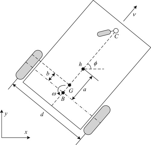
For the model shown in the figure, G is the mass centre of the mobile robot; h denotes the simplified point of the mobile robot in the x–y plane, whose coordinates are indicated as $(x,y)$; ϕ represents the directional angle of the mobile robot; a indicates the distance between h and B, where B is the axis centre of the wheels; b is the distance from G to B; d is the distance of two rear wheels; and C is a caster to balance the mobile robot. Note that, in the rest of this paper, the time variable t of the variables is omitted for simplicity except special indication.

Bearing the DDMR model in mind, the kinematic model can be obtained via the kinematic analysis as follows Khai et al. (2020) (1) $\begin{array}{r}\left[\begin{array}{c}\dot{x}\\ \dot{y}\\ \dot{\varphi }\end{array}\right]=\left[\begin{array}{cc}\cos \varphi & -a\sin \varphi \\ \sin \varphi & a\cos \varphi \\ 0& 1\end{array}\right]\left[\begin{array}{c}\nu \\ \omega \end{array}\right],\end{array}$(1) where ω and ν stand for the angular and linear velocities of the mobile robot.

2.2. Dynamic model of the mobile robot

Through the force analysis and the moment analysis for the mass centre G of the mobile robot, the dynamic model of the DDMR can be yielded via dynamic analysis as Martins et al. (2016) (2) $\begin{array}{r}\left[\begin{array}{c}\dot{\nu }\\ \dot{\omega }\end{array}\right]=\left[\begin{array}{c}{\displaystyle \frac{{\theta }_3}{{\theta }_1}{\omega }^2-{\displaystyle \frac{{\theta }_4}{{\theta }_1}\nu }}\\ [6pt]-{\displaystyle \frac{{\theta }_5}{{\theta }_2}\nu \omega -{\displaystyle \frac{{\theta }_6}{{\theta }_2}\omega }}\end{array}\right]+\left[\begin{array}{cc}{\displaystyle \frac{1}{{\theta }_1}}& 0\\ [6pt]0& {\displaystyle \frac{1}{{\theta }_2}}\end{array}\right]\left[\begin{array}{c}{u}_{\nu }\\ u_{\omega }\end{array}\right]+\left[\begin{array}{c}{\delta }_{\nu }\\ {\delta }_{\omega }\end{array}\right],\end{array}$(2) where $[{\delta }_{\nu },{\delta }_{\omega }{]}^{\mathrm{T}}$ is the vector indicating the uncertainty of ν and ω; $u_{\nu }$ and $u_{\omega }$, the reference velocities, can be taken as the control inputs of the mobile robot. The dynamic parameters ${\theta }_1$–${\theta }_6$ of the DDMR can be calculated as follows: (3) $\begin{array}{r}\begin{array}{rl}{\theta }_1& =\frac{\frac{R_a}{k_a}(m{R}_{t}r+2I_e)+2r{k}_{DT}}{2r{k}_{PT}},\\ {\theta }_2& =\frac{\frac{R_a}{k_a}(I_e{d}^2+2R_{t}r(I_z+m{b}^2))+2rd{k}_{DR}}{2rd{k}_{PR}},\\ {\theta }_3& =\frac{R_a}{k_a}\frac{mb{R}_t}{2k_{PT}},\\ {\theta }_4& =\frac{\frac{R_a}{k_a}(\frac{k_a{k}_b}{R_a}+B_e)}{r{k}_{PT}}+1,\\ {\theta }_5& =\frac{R_a}{k_a}\frac{mb{R}_t}{d{k}_{PR}},\\ {\theta }_6& =\frac{R_a}{k_a}\left(\frac{k_a{k}_b}{R_a}+B_e\right)\frac{d}{2r{k}_{PR}}+1.\end{array}\end{array}$(3) As observed in the above expressions, the dynamic parameters can be determined by some physical parameters of the mobile robot, including the mass m, the moment of inertia $I_z$ at point G, the electrical resistance $R_a$ of the motors, the electromotive constant $k_b$ of the motors, the torque constant $k_a$ of the motors, the coefficient of friction $B_e$, the moment of inertia $I_e$ of the motor-gear-wheel system, the radius of the wheels r, and the distances b and d, etc. Due to page limits, we refer the interested readers to Khai et al. (2020) and Martins et al. (2016) for more details of the modelling of the differential-drive mobile robot mentioned above.

3. Design of trajectory tracking control system for differential-drive mobile robot

3.1. Structure of the control system

In this paper, a scheme combined with backstepping and FOPID is proposed for the trajectory tracking of mobile robots, and the control system has been displayed in Figure 2.

Figure 2. Control system for the trajectory tracking of DDMR.

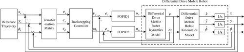
As depicted in Figure 2, the real pose ($x,y,\varphi$) of the mobile robot is compared with its reference values ($x_r,y_r,{\varphi }_r$) to obtain the pose error ($e_x,e_y,e_{\varphi }$), which is used to produce the designed velocity instructions (i.e. the kinematic control law $[{\nu }_d,{\omega }_d]$) through the backstepping controller. Then, the FOPID controllers are employed to regulate the velocity errors of the mobile robot, and the outputs of the controllers (i.e. the dynamic control law $[u_{\nu },u_{\omega }]$) are exerted to control the mobile robot.

In the remainder of this section, the design of the kinematic and the dynamic controllers has been described in detail respectively.

3.2. Design of the kinematic backstepping controller

Backstepping is a scheme for the nonlinear system controller design based on Lyapunov theory (Mai et al., 2021). The scheme of backstepping is to decompose the complex nonlinear system into several subsystems, and the Lyapunov functions and virtual variables of the subsystems are designed iteratively for the control law of the whole system.

For the mobile robot sketched in Figure 1, the pose errors can be expressed as Yue et al. (2012) (4) $\begin{array}{r}\left[\begin{array}{c}{e}_x\\ e_y\\ e_{\varphi }\end{array}\right]=\left[\begin{array}{ccc}\cos \varphi & \sin \varphi & 0\\ -\sin \varphi & \cos \varphi & 0\\ 0& 0& 1\end{array}\right]\left[\begin{array}{c}{x}_r-x\\ y_r-y\\ {\varphi }_r-\varphi \end{array}\right],\end{array}$(4) whose dynamic function can be calculated as (5) $\begin{array}{r}\left[\begin{array}{c}{\dot{e}}_x\\ {\dot{e}}_y\\ {\dot{e}}_{\varphi }\end{array}\right]=\left[\begin{array}{c}\omega e_y-\nu +{\nu }_r\cos e_{\varphi }\\ {\nu }_r\sin e_{\varphi }-\omega e_x\\ {\omega }_r-\omega \end{array}\right].\end{array}$(5) First, we consider the following Lyapunov function (6) $\begin{array}{r}{L}_1=\frac{e_x^2+e_y^2}{2},\end{array}$(6) where $L_1\ge 0$ and we can get (7) $\begin{array}{rl}{\dot{L}}_1& =e_x{\dot{e}}_x+e_y{\dot{e}}_y\\ & =e_x(\omega e_y-\nu +{\nu }_r\cos e_{\varphi })+e_y({\nu }_r\sin e_{\varphi }-\omega e_x)\\ & =-\nu e_x+{\nu }_r{e}_x\cos e_{\varphi }+{\nu }_r{e}_y\sin e_{\varphi }.\end{array}$(7) Take the virtual control law of ν as (8) $\begin{array}{r}\nu =k_1{e}_x+{\nu }_r\cos e_{\varphi },\end{array}$(8) then (9) $\begin{array}{r}{\dot{L}}_1=-k_1{e}_x^2+{\nu }_r{e}_y\sin e_{\varphi }.\end{array}$(9) Moreover, we consider the following Lyapunov function with $k_2>0$ (10) $\begin{array}{r}L=L_1+\frac{1-\cos e_{\varphi }}{k_2},\end{array}$(10) and we can get (11) $\begin{array}{rl}\dot{L}& =-k_1{e}_x^2+{\nu }_r{e}_y\sin e_{\varphi }+\frac{{\dot{e}}_{\varphi }}{k_2}\sin e_{\varphi }\\ & =-k_1{e}_x^2+{\nu }_r{e}_y\sin e_{\varphi }+\frac{{\omega }_r-\omega }{k_2}\sin e_{\varphi }.\end{array}$(11) In order to obtain an asymptotic stability system, we let $\dot{L}\le 0$, then the virtual control law of ω can be yielded as (12) $\begin{array}{r}\omega ={\omega }_r+k_2{\nu }_r{e}_y.\end{array}$(12) Then the kinematic control law can be expressed as follows: (13) $\begin{array}{r}\left[\begin{array}{c}{\nu }_d\\ {\omega }_d\end{array}\right]=\left[\begin{array}{c}{k}_1{e}_x+{\nu }_r\cos e_{\varphi }\\ {\omega }_r+k_2{\nu }_r{e}_y\end{array}\right],\end{array}$(13) where $[{\nu }_r,{\omega }_r]$ are the linear and angular reference velocities of the mobile robot; $[{\nu }_d,{\omega }_d]$ are the output of the backstepping controller; and $k_1>0,k_2>0$ are two parameters to be designed for the kinematic controller.

3.3. Design of the dynamic FOPID controller

In this section, the FOPID controller is designed for the dynamic control of the mobile robot, where the Grunwald-Letnikov definition for the fractional calculus is utilized and expressed as follows Xu et al. (2019): (14) $\begin{array}{r}{}_{t_0}{\mathcal{D}}_t^{\lambda }f(t)=\underset{h\to 0}{lim}{h}^{-\lambda }\sum _{k=0}^{[\frac{t-t_0}{h}]}(-1{)}^k\left(\begin{array}{c}\lambda \\ j\end{array}\right)f(t-kh),\end{array}$(14) where $[\cdot ]$ denotes the rounding operation; h indicates the step of the numerical calculation; and the differential operator ${}_{t_0}{\mathcal{D}}_t^{\lambda }$ is defined as follows: (15) $\begin{array}{r}{}_{t_0}{\mathcal{D}}_t^{\lambda }=\{\begin{array}{ll}{\mathrm{d}}^{\lambda }/\mathrm{d}{t}^{\lambda }& \lambda >0,\\ 1& r=0,\\ {\displaystyle {\int }_{t_0}^t(\mathrm{d}\tau {)}^{-\lambda }}& \lambda <0,\end{array}\end{array}$(15) where $\lambda \in \mathbb{R}$ denotes the fractional order; $t_0$ and t stands for the lower and upper limits of the operator respectively.

For the sake of simplicity in implementation, the fractional differential operator in this paper is approximated by a modified Oustaloup filter with a frequency band of $({\omega }_b,{\omega }_h)$ expressed as follows Xue et al. (2006): (16) $\begin{array}{r}{s}^{\lambda }\approx {\left(\frac{\mathrm{d}{w}_h}{b}\right)}^{\lambda }\left(\frac{b{w}_{h}s+\mathrm{d}{s}^2}{\mathrm{d}\lambda +b{w}_{h}s+\mathrm{d}(1-\lambda )s^2}\right)\prod _{k=1}^N\frac{s+w_k^{\mathrm{\prime }}}{s+w_k},\end{array}$(16) where $w_k=w_b{w}_u^{\frac{2k-1+\lambda }{N}}$, ${w_k}^{\mathrm{\prime }}=w_b{w}_u^{\frac{2k-1-\lambda }{N}}$, $w_u=\sqrt{\frac{w_h}{w_b}}$; N is the order of the filter; λ is the fractional order of the differential operator; $w_h$ and $w_b$ indicate respectively the lower and upper limits of the selected fitting frequency; and the parameters b and d are usually set as 10 and 9.

For the dynamic control of the mobile robot, we use the fractional-order PID controller expressed as follows 2017: (17) $\begin{array}{r}u(t)=k_{p}e(t)+k_i{\mathcal{D}}^{-\lambda }e(t)+k_d{\mathcal{D}}^{\mu }e(t),\end{array}$(17) whose Laplace transform can be expressed as (18) $\begin{array}{r}C(s)=k_p+\frac{k_i}{s^{\lambda }}+k_d{s}^{\mu },\end{array}$(18) where $u=[u_{\nu },u_{\omega }]$ are the output of the dynamic controller, $e=[e_{\nu },e_{\omega }]$ are the errors for the linear and angular velocities of the mobile robot, where the time variable t is omitted for simplicity; $k_p$, $k_i$, $k_d$, λ and μ are the parameters to be tuned for the FOPID controller. The structure of the FOPID controller is described in Figure 3, and two FOPID controllers are exploited to regulate the velocities of the mobile robot respectively as depicted in Figure 2.

Figure 3. Dynamic controller of DDMR based on FOPID.

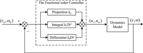
Remark 3.1

It is worth noting that the traditional PID controller is a special case of the FOPID controller with $\lambda =1$ and $\mu =1$. By tuning the two additional controller parameters, the performance of FOPID controller can be greatly promoted and outperform the traditional PID controller in the trajectory tracking control of mobile robots.

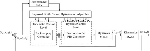
It should be highlighted that there are several parameters to be designed in the control system of the mobile robot. In order to obtain the optimal trajectory tracking controller, the parameters should be optimized in terms of some performance criteria. Unfortunately, the optimization of these parameters is an intractable problem due to some frequently appeared obstacle phenomena in the optimization. To circumvent this difficulty, an improved intelligent optimization algorithm is developed in the next section of this paper.

4. Control system optimization based on improved beetle swarm optimization algorithm

In Jiang and Li (2017), Jiang and his colleague proposed a new intelligent optimization algorithm, beetle antennae search (BAS) algorithm, whose idea comes from the foraging behaviour of the beetle antennae (BA). In the process of foraging, the beetle antennae can determine its next step close to the food by detecting the smell intensity. The BAS algorithm imitates the search behaviour of the beetle antennae in the optimization problem, and can quickly find an optimal solution with low computation cost.

Particle swarm optimization (PSO) algorithm is another intelligent optimization algorithm mimics the foraging behaviour of bird swarms or fish schools (Xu et al., 2021). By using a large number of particles flying randomly in the search space, the PSO algorithm can freely explore the search space to obtain an optimal solution.

In contrast, the BAS algorithm is an expert in exploiting the search space, but the one beetle antennae based BAS algorithm is prone to local trapping and suboptimal solution. The PSO algorithm has better performance in the exploration of the search space, while it is inferior to BAS in terms of exploitation ability. Hence, it is a natural motive to combine the advantages of PSO and BAS, and this results in the beetle swarm optimization (BSO) algorithm proposed in T. Wang et al. (2020).

In BSO, the particles in PSO are replaced by several BAs, whose position and velocity updating schemes are similar to the particles in PSO. The updating functions of BSO are expressed as follows: (19) $\begin{array}{rl}& {\xi }_i^{t+1}={\xi }_i^t+{\delta }^t\overrightarrow{b}\mathrm{sgn}((f(x_{ri}^t)-f(x_{li}^t))),\end{array}$(19) (20) $\begin{array}{rl}& v_i^{t+1}=w{v}_i^t+c_1{r}_{i1}(P_i^t-x_i^t)+c_2{r}_{i2}(G^t-x_i^t),\end{array}$(20) (21) $\begin{array}{rl}& x_i^{t+1}=x_i^t+\lambda v_i^{t+1}+(1-\lambda ){\xi }_i^{t+1},\end{array}$(21) where ${\xi }_i^t$ denotes the current step of the ith beetle, whose current velocity and position are indicated by $v_i^t$ and $x_i^t$ respectively; the updating scheme of velocity $v_i^t$ is compatible with PSO, and the position $x_i^t$ is updated with the λ weighted $v_i^{t+1}$ and ${\xi }_i^{t+1}$; ${\delta }^t$ is the search step of the beetle in the current iteration and updated as follows: (22) $\begin{array}{r}{\delta }^{t+1}={\delta }_e{\delta }^t,\end{array}$(22) where ${\delta }_e$ is a degradation factor of ${\delta }^t$; $\overrightarrow{b}$ is a normalized vector that can be calculated as (23) $\begin{array}{r}\overrightarrow{b}=\frac{\mathrm{rands}(k,1)}{\Vert \mathrm{rands}(k,1)\Vert },\end{array}$(23) where $\mathrm{rands}(\cdot )$ produces a k-dimensional random vector; $f(\cdot )$ is the fitness function of $x_{ri}^t$ and $x_{li}^t$, which are the positions of the right and left antennaes of the ith beetle and can be calculated as follows: (24) $\begin{array}{rl}& x_{ri}^t=x_i^t-d^{t+1}\overrightarrow{b},\end{array}$(24) (25) $\begin{array}{rl}& x_{li}^t=x_i^t+d^{t+1}\overrightarrow{b},\end{array}$(25) where d is the distance between two antennaes and is updated as (26) $\begin{array}{r}{d}^{t+1}=d_e{d}^t,\end{array}$(26) where $d_e$ is a degradation factor of $d^t$.

In BSO, the inertia weight w is a critical parameter to the optimization result. For example, a large w can enhance the global exploration ability of BSO, and a small w would achieve the better exploitation performance. Thus, we use a nonlinear iterative function to improve the BSO algorithm, whose inertia weight is updated as follows: (27) $\begin{array}{r}w=\frac{w_{max}-w_{min}}{2}\cos \left(\pi {\left(\frac{t}{T_{max}}\right)}^2\right)+\frac{w_{max}+w_{min}}{2},\end{array}$(27) where $w_{max}$ and $w_{min}$ are respectively the maximum and minimum values of w; and $T_{max}$ is the maximum iteration.

Now, we use the improved BSO algorithm for the optimization of the DDMR control system. Specifically, the parameters of the kinematic backstepping controller and the dynamic FOPID controller are tuned based on the ITAE criteria expressed as follows: (28) $\begin{array}{r}min{J}_{\mathrm{ITAE}}={\int }_0^{\mathrm{\infty }}t|e(t)|\mathrm{d}t,\end{array}$(28) where $e(t)=\sqrt{(x_r-x{)}^2+(y_r-y{)}^2}$ is the position error of the trajectory tracking control. The optimization of the control system is sketched in Figure 4.

Figure 4. Optimization of control system based on BSO.

5. Simulation results

In this section, some simulation results are reported to verify the effectiveness and superiority of the proposed trajectory tracking controller.

In the simulation, the parameters of the DDMR model are set as follows: ${\theta }_1=0.3625$, ${\theta }_2=0.2609$, ${\theta }_3=-0.0005$, ${\theta }_4=1.0122$, ${\theta }_5=0.0031$, ${\theta }_6=1.0986$. For the dynamic control of the DDMR, we compare the effect of the PID and FOPID controllers whose parameters are tuned by the improved BSO algorithm. The configuration of the BSO algorithm is set as follows: $w_{max}=0.9$, $w_{min}=0.4$, $c_1=c_2=2$, $\lambda =0.4$, $d_e={\delta }_e=0.95$.

The initial position of the DDMR is set as $(0.2,0)$, and the reference trajectory for the DDMR to track is a 8-shape trajectory expressed as follows: (29) $\begin{array}{rl}& x_r(t)=A_x\sin (2ft)\end{array}$(29) (30) $\begin{array}{rl}& y_r(t)=A_y\sin (ft)\end{array}$(30) where f = 0.04, $A_x=A_y=1$. In the case of no skidding and sliding of the wheels, the tracking results of the two controllers are shown in Figures 5 and 6, where the red dotted line is the reference trajectory and the blue line is the actual trajectory of the mobile robot. The trajectory tracking errors are compared and shown in Figure 7, where the results of PID and FOPID based control systems are manifested by red and blue lines respectively. Then, considering the skidding and sliding of the wheels, we set the random skidding velocity with maximum value ${\nu }_s=0.05\mathrm{m}/\mathrm{s}$ and the random sliding velocity of two wheels with maximum value ${\nu }_{sr}={\nu }_{sl}=0.02\mathrm{m}/\mathrm{s}$. The robustness of the trajectory tracking control system can be demonstrated by the simulation results shown in Figures 8 and 9, and the trajectory tracking errors are compared and shown in Figure 10. It is obvious that the FOPID based control system can obtain smaller position tracking error than the PID based control system.

Figure 5. Trajectory tracking result based on PID controller (no skidding and sliding).

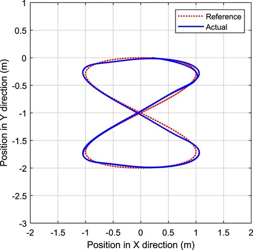
Figure 6. Trajectory tracking result based on PI${}^{\lambda }$D${}^{\mu }$ controller (no skidding and sliding).

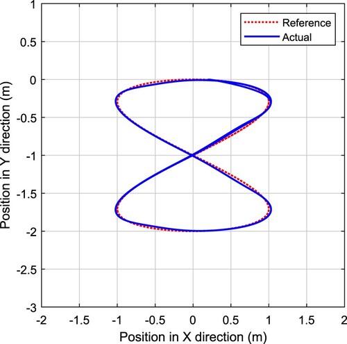
Figure 7. Comparison of trajectory tracking errors (no skidding and sliding).

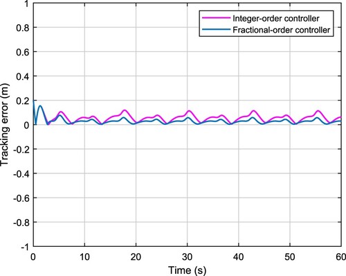
Figure 8. Trajectory tracking result based on PID controller (with skidding and sliding).

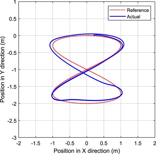
Figure 9. Trajectory tracking result based on PI${}^{\lambda }$D${}^{\mu }$ controller (with skidding and sliding).

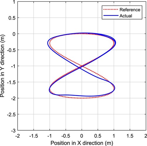
Figure 10. Comparison of trajectory tracking errors (with skidding and sliding).

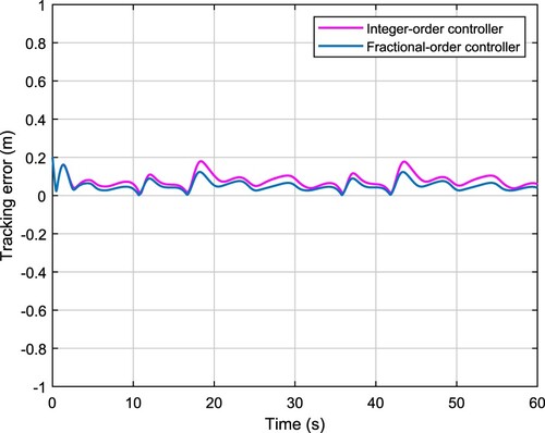
From the simulation results, we can conclude that, on the one hand, the control scheme combined with backstepping and FOPID is effective for the trajectory tracking of the mobile robot in both cases with and without skidding and sliding; on the other hand, the FOPID can outperform the PID on the dynamic control for the trajectory tracking of the mobile robot. Note that, all the control systems in comparison are optimized by the improved BSO algorithm, and the superior performance of FOPID based scheme is benefited from two additional tunable controller parameters.

6. Conclusions

In this paper, based on the kinematic and the dynamic models of the mobile robot, a control scheme combined with backstepping and FOPID is developed for the trajectory tracking of mobile robots. In order to optimize the control system, an improved BSO algorithm is presented to tune the parameters of the kinematic and the dynamic controllers based on the ITAE criteron simultaneously. Several simulations are implemented for the trajectory tracking of mobile robot in the cases with and without skidding and sliding. The simulation results can verify the effectiveness and superiority of the combined control scheme developed in this paper.

In the future work, we will focus on some interesting topics, such as networked mobile robot control in complex environment (Zou, Wang, Hu, et al., 2020; Zou, Wang, & Zhou, 2020) and trajectory tracking control of the omnidirectional mobile robot (Sira-Ramirez et al., 2013), etc.

Disclosure statement

No potential conflict of interest was reported by the author(s).

Additional information

Funding

This work was supported in part by the National Natural Science Foundation of China [grant number 61703242] and the Natural Science Foundation of Shandong Province China [grant number ZR2020MF071].

References

- Gheisarnejad, M., & Khooban, M. H. (2021). An intelligent non-integer PID controller-based deep reinforcement learning: Implementation and experimental results. IEEE Transactions on Industrial Electronics, 68(4), 3609–3618. https://doi.org/10.1109/TIE.41
- Huang, H. C., & Chiang, C. H. (2016). Backstepping holonomic tracking control of wheeled robots using an evolutionary fuzzy system with qualified ant colony optimization. International Journal of Fuzzy Systems, 18(1), 28–40. https://doi.org/10.1007/s40815-015-0106-4
- Jiang, X., & Li, S. (2017). BAS: Beetle antennae search algorithm for optimization problems. International Journal of Robotics and Control, 1(1), 1–5. https://doi.org/10.5430/ijrc.v1n1p1
- Khai, T., Ryoo, Y., & Gill, W. (2020). Design of kinematic controller based on parameter tuning by fuzzy inference systems for trajectory tracking of differentia-drive mobile robot. International Journal of Fuzzy Systems, 22(7), 1–7. https://doi.org/10.1007/s40815-020-00842-9
- Li, S., Wang, Q., & Ding, L. (2020). Adaptive NN-based finite-time tracking control for wheeled mobile robots with time-varying full state constraints. Neurocomputing, 403(2), 421–430. https://doi.org/10.1016/j.neucom.2020.04.104
- Mai, T. A., Dang, T. S., & Duong, D. T. (2021). A combined backstepping and adaptive fuzzy PID approach for trajectory tracking of autonomous mobile robots. Journal of the Brazilian Society of Mechanical Sciences and Engineering, 43(3), 1–13. https://doi.org/10.1007/s40430-020-02767-8
- Martins, F., Sarcinelli-Filho, M., & carelli, R. (2016). A velocity-based dynamic model and its properties for differential drive mobile robots. Journal of Intelligent and Robotic Systems, 85(2), 277–292. https://doi.org/10.1007/s10846-016-0381-9
- Saleh, A., Hussain, M., & Klim, S. (2018). Optimal trajectory tracking control for a wheeled mobile robot using fractional-order-PID-controller. Journal of University of Babylon for Engineering Sciences, 26(4), 292–306. https://doi.org/10.29196/jubes.v26i4.1087
- Sen, P. T. H., Minh, N. Q., A, D. T. T., & Minh, P. X. (2019). A new tracking control algorithm for a wheeled mobile robot based on backstepping and herarchical sliding mode techniques. In Proceedings of First International Symposium on Instrumentation, Control, Artificial Intelligence, and Robotics (pp. 25–28). IEEE.
- Sira-Ramirez, H., Lopez-Uribe, C., & Velasco-Villa, M. (2013). Linear observer-based active disturbance rejection control of the omnidirectional mobile robot. Asian Journal of Control, 15(1), 51–63. https://doi.org/10.1002/asjc.v15.1
- Waleed, A. O., & Hadi, A. N. (2018). Design and stability analysis of a fractional order state feedback controller for trajectory tracking of a differential drive robot. International Journal of Control, Automation and Systems, 16(6), 2790–2800. https://doi.org/10.1007/s12555-017-0234-8
- Wang, J., Lu, Z., Chen, W., & Wu, X. (2011). An adaptive trajectory tracking control of wheeled mobile robots. In Proceedings of 6th IEEE Conference on Industrial Electronics and Applications (pp. 1156–1160). IEEE.
- Wang, T., Yang, L., & Liu, Q. (2020). Beetle swarm optimization algorithm: Theory and application. Filomat, 34(15), 5121–5137. https://doi.org/10.2298/FIL2015121W
- Wang, X., Zhang, G., & Neri, F. (2015). Design and implementation of membrane controllers for trajectory tracking of non-holonomic wheeled mobile robots. Integrated Computer-Aided Engineering, 23(1), 15–30. https://doi.org/10.3233/ICA-150503
- Xu, L., Song, B., & Cao, M. (2021). An improved particle swarm optimization algorithm with adaptive weighted delay velocity. Systems Science & Control Engineering, 9(1), 188–197. https://doi.org/10.1080/21642583.2021.1891153
- Xu, L., Song, B., Cao, M., & Xiao, Y. (2019). A new approach to optimal design of digital fractional-order PI λD μ controller. Neurocomputing, 363(6), 66–77. https://doi.org/10.1016/j.neucom.2019.06.059
- Xue, D., Zhao, C., & Chen, Y. Q. (2006). A modified approximation method of fractional order system. In Proceedings of the 2006 IEEE International Conference on Mechatronics and Automation (pp. 1043–1048). IEEE.
- Yue, M., Tang, F., Liu, B., & Yao, B. (2012). Trajectory-tracking control of a nonholonomic mobile robot: Backstepping kinematics into dynamics with uncertain disturbances. Applied Artificial Intelligence, 26(10), 952–966. https://doi.org/10.1080/08839514.2012.731347
- Zhang, L., Liu, L., & Zhang, S. (2020). Design, implementation, and validation of robust fractional-order PD controller for wheeled mobile robot trajectory tracking. Complexity, 2020(4), 1–12. https://doi.org/10.1155/2020/9523549
- Zhao, H., Song, B., Zhang, J., & Xu, L. (2017). Fractional order PID controller design based on PSO algorithm. Journal of Shandong University of Science and Technology (Natural Science), 36(4), 60–65.
- Zou, L., Wang, Z., Hu, J., & Zhou, D. H. (2020). Moving horizon estimation with unknown inputs under dynamic quantization effects. IEEE Transactions on Automatic Control, 65(12), 5368–5375. https://doi.org/10.1109/TAC.9
- Zou, L., Wang, Z., & Zhou, D. H. (2020). Moving horizon estimation with non-uniform sampling under component-based dynamic event-triggered transmission. Automatica, 120(3), Article number 109154. https://doi.org/10.1016/j.automatica.2020.109154