The impact of livelihood diversification as a climate change adaptation strategy on poverty level of pastoral households in southeastern and southern Ethiopia

Abstract

The purpose of this study was, therefore, to examine the determinants of poverty depth in pastoral households, and the impact of adopting livelihood diversification on the poverty level of households in the Arero district of Borena Zone and Rayitu district of Bale Zone, Ethiopia. A multistage sampling technique was used, and 396 households were selected from the Arero and Rayitu Districts. The cost of basic needs (CBN) approach was used to determine the study areas. Accordingly, the absolute poverty line was determined to be 10,881.26 Birr per adult per annum. Based on the poverty line, 34.6 % of the sample households were in the poor category. The Foster-Greer-Thorbecke index results indicated that the poverty incidence, poverty gap, and poverty severity were 34.6, 9.28, and 3.62, respectively. Two econometric models were used for the analysis, namely the Tobit and Multinomial Endogenous Switching models. The results of the Tobit logistic regression revealed that the age of the household head, household size, and distance to the nearest market significantly increased the poverty level of the pastoral households. However, livestock size as measured by tropical livestock unit and frequency of extension contact significantly decreased the poverty depth of pastoral households. On the other hand, the output of the multinomial endogenous switching regression model showed that the joint adoption of non-farm activities and crop production had a decreasing and significant impact on the poverty level of pastoral households. Therefore, policies that promote livelihood diversification of pastoral communities are critical to lowering the poverty level of pastoral households in semi-arid areas.

Keywords:

• poverty
• poverty line
• Foster-Greer-Thorbecke Index
• livelihood diversification
• determinants, impact, Ethiopia

1. Introduction

It has been a number of years since climate change was recognized as one of the greatest threats to our world. Since the industrial revolution, the world has begun to notice climate change, which is one of the unfavorable effects of global warming. For instance, the average global temperature increased by 1.1 degrees Celsius until 2017 compared to the pre-industrial era (WMO, 2018). According to Guilyardi et al. (2018), the increase in global temperature will probably exceed 1.5 degrees Celsius between 2030 and 2052 if greenhouse gas emissions continue at their current rates.

Unpredictably, the effects of climate change are felt worldwide. However, dry and semi-arid rangelands, which make about 30% of the world’s land area, have recently been severely impacted by the effects of climate change (Galvin et al., 2001; Herrero et al., 2016; Malagnoux, 2007). The increased susceptibility of pastoral communities in these areas to chronic hunger and poverty is an effect of climate change. According to FAO (2018), recurring and overlapping climate shocks make pastoralist populations in Africa’s arid plains more susceptible to hunger, famine, and high rates of acute malnutrition.

Pastoralist households in Ethiopia also use various adaptation strategies to cope with the adverse effects of climate change and its variability. These include water harvesting systems, fodder production, increased mobility, restocking of livestock, and diversification of livestock herds in favor of a drought-tolerant species (camel) (Berhanu & Beyene, 2014; Melaku et al., 2017). In addition, pastoralist communities in the country have adopted a range of livelihood diversification strategies to combat the effects of climate change, including crop production, wage labor, petty trading, fuelwood and charcoal production (Birhanu & Getachew, 2017). Similarly (Maxwell, 2017), argued that options for diversified livelihood activities are limited in pastoral areas, and poorer people in particular have few options and are forced to engage in low-income or low-wage activities and/or activities with negative long-term environmental or social impacts.

There has been a major loss of crops and animals due to climate change in sub-Saharan African countries, which has led to widespread food insecurity and poverty in the area. According to a study conducted in Tanzania, severe recurrent drought periods caused a lack of forage and water, which caused the cattle to starve and become malnourished. Mass cattle deaths and disease outbreaks have also had a significant impact on the livelihood of pastoral communities in northern Tanzania (Kimaro et al., 2018). Similarly, Food for the Hungry and Tearfund (2019) reported that, over time, the livelihoods of pastoralist communities in Kenya have been severely impacted by recurring droughts. Such climate-related shocks are becoming more severe and more frequent, and the prolonged drought alone wiped out approximately 60% of the county’s livestock population in 2017. According to academics, poverty reduction in Africa, notably sub-Saharan Africa, has been uneven and has lagged behind other developing parts of the world (Anyanwu & Anyanwu, 2017).

The main causes of poverty in sub-Saharan Africa can be traced to various sources. High income inequality, institutionalized democracy, corruption, poor governance, low employment prospects, inadequate infrastructure, inefficient use of resources, an increase in civil war episodes, and an endless cycle of conflict are some of these (Addae-Korankye, 2014; Anyanwu & Anyanwu, 2017). In turn, income inequality in the region is caused by underlying factor endowments, the location of much of the land area in the tropics, suboptimal structural transformation of the economy, and unequal distribution of socioeconomic and physical capital capitals (UNDP, 2017)

Although Ethiopia’s economy has expanded significantly across all sectors, the country’s food insecurity and poverty problems have not been resolved. Chronic malnutrition, acute poverty, a young population that is expanding quickly and is unemployed in both urban and rural areas, civil and political tensions, and escalating droughts are making it difficult for the nation to address widespread well-being problems (Feed the Future, 2018). In 2015, the country faced one of the worst droughts in decades, resulting in over 10.2 million people needing food assistance in 2016, down to 7.9 million in 2018 (UNICEF, 2015, 2018). In addition, it is estimated (USAID, 2020) that about 8.4 million people needed humanitarian assistance nationwide in 2020, as violence, erratic rains, pest infestations, and disease outbreaks negatively affect the lives and livelihoods of vulnerable people.

Lowland pastoralists and agro-pastoralists in Ethiopia are among the most vulnerable to the impacts of climate change and variability. Studies carried out in the nation have revealed that cattle health, reproduction, and mortality rates are affected by climate change and climate variability, as manifested by rising temperatures and decreasing rainfall along with its unpredictable distribution (Desalegn et al., 2018; Mikias, 2014). Therefore, livestock health is affected by climate change and variability, which results in decreased productivity and animal deaths, increasing the vulnerability of pastoralist communities in the country to food insecurity and poverty.

Therefore, to combat the negative consequences of climate change that threaten their well-being and sustainable livelihoods, pastoral communities must use various adaptation techniques. One technique that vulnerable individuals can adopt to safeguard their current livelihood systems, diversify their sources of income, and alter their livelihood strategies to strengthen their resilience. In accordance with Berhanu and Beyene (2014), pastoralists’ perceptions of climate change are consistent with the actual recorded trends of rising temperatures and an obvious secular decline in precipitation. Pastoralist adaptation response strategies typically involve modifications of pastoral practices and a shift to non-pastoral livelihoods.

Studies conducted in various pastoral and agropastoral regions of Ethiopia have shown that poverty is a common occurrence. The specific studies conducted by Teka et al. (2019) and Shibru et al. (2014) revealed that the poverty gap of poverty in rural areas is high, which is influenced by factors such as the gender of the household head, family size, farm land size, non-farm activities, educational status, livestock holding, herd diversification, distance from market center, farm income, and non-farm income.

According to previous studies, the effects of climate change are endangering the population of Ethiopia by worsening its level of poverty. According to (Tagesse et al., 2020), various livelihood diversification techniques have made a significant difference in reducing a nation’s poverty problem. This shows that as a strategy for coping with climate change, livelihood diversification plays a significant role in lowering poverty level in the country’s poverty level.

The causes of poverty among pastoral and agro-pastoral households in Ethiopia have been the subject of several empirical studies. For instance, using a logit regression model (Araya et al., 2019), examined the factors influencing the poverty of pastoral and agro-pastoral households in the Afar Regional State of Ethiopia. In addition, a different study was conducted in the same region’s Abysaita District using the Tobit regression model to determine the variables that influence the poverty level of agro-pastoral households (Abubeker et al., 2014). Additionally (Shibru et al., 2014), employed a binary logit model to uncover factors that determine poverty status in agro-pastoral communities in the Dembel District of the Somali Regional State of Ethiopia.

In addition, empirical studies have been conducted on the impact of livelihood diversification on poverty at the rural household level in Ethiopia. For example (Tsehaynesh et al., 2021), investigated the impact of livelihood diversification on rural poverty using propensity score matching in Jimma Zone, Oromia National Regional State, Southwest Ethiopia, Ethiopia. The results show that livelihood diversification had a positive impact on poverty among rural households that participated in livelihood diversification. A study of the impact of crop diversification as a climate change adaptation strategy on agricultural income using ESRM in the Nile Basin of Ethiopia also showed a positive result (Fissha et al., 2019). However, none of these studies specifically examined the effects of livelihood diversification on rural poverty at the household level among pastoral households in semi-arid regions. Therefore, the study aimed to Therefore, the study aimed at 1) identify the trends of climate variables, temperatures and rainfall in the study areas; (2)examining the poverty incidence, poverty gap and poverty severity using the Foster-Greer-Thorbecke index; (3) identifying factors affecting the depth of poverty of the pastoral households (4) quantifying the impact of pastoralists’ livelihood diversification on the poverty level of the pastoralist households using the multinomial switching regression model in semi-arid areas

2. Materials and methods

2.1. Descriptions of the study areas

The study was conducted in the districts of Arero in the Borena Zone, which is in the southern part of Ethiopia, and Rayitu in the Bale Zone, which is in the southeast. The Bale Zone is geographically located between 5.36° N-8.12° N and 39.21° E-42.23° E (Fitsum et al., 2017). It is bordered by the Somali National Regional State of Ethiopia in the East, East Hararge zone in the Northeast, West Hararge and Arsi zones in the North, West Arsi Zone in the West, and Guji Zone in the Southwest (Figure 1). The eastern part of the zone is characterized by semi-desert climatic conditions and is inhabited by pastoral communities.

Figure 1. Location of the study areas.

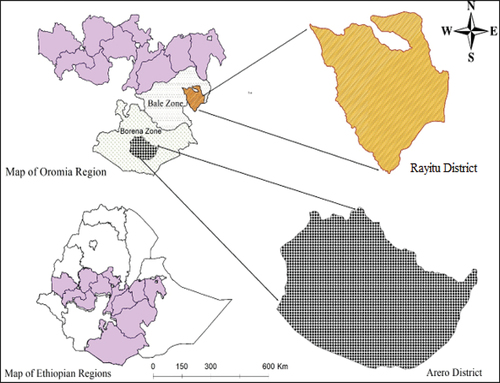
Geographically, the Borena Zone is situated between 4º and 6º N latitude and 36º to 42º E longitude in the southern region of the nation (Dereje et al., 2022). It is surrounded by Kenya to the south; the Somali area to the southeast; the Southern Nation, Nationalities, and People (SNNP) to the west; and the West Guji Zone to the north (Figure 1). The region is mostly distinguished by its semi-arid climate, which has two rainy seasons, an average annual rainfall that varies between 350 mm and 1100 mm, and mean annual temperature of 19°C (Debela et al., 2019; Desalegn et al., 2018; Mitiku et al., 2022).

Rayitu District is one of the districts in the eastern part of the Bale Zone. The district is bordered by Sewena in the east and north, Ginnir in the west, and the Somali regional state in the south. It is bordered by three perennial rivers: Wabi Shebele, Weyib, and Dinikte. This district is one of the pastoralist community-dominated districts of the Bale Zones. The long rainy season lasts from March to June, whereas the short rainy season lasts from September to October, with an average annual rainfall of approximately 450 mm (Mohammed et al., 2018). It is prone to drought and has a bimodal rainfall pattern and erratic distribution. The district is characterized by hot, dry weather, with an average annual temperature of 26°C, and it lies within an altitudinal range of 500 and 1,785 meters above sea level (Serkalem et al., 2014).

Arero is one of the districts in the Borena Zone, which is dominated by pastoral and agro-pastoral communities. Geographically, the Arero District is situated at 4 °45’0’ N and 38 °490’E, 650 km south of Addis Ababa (Aden & Kula, 2020). As seen in Figure 1, it shares borders with the Somali area to the east, Guji zone to the northeast, Bule Hora district to the north, Yabelo district to the west, Dire district to the southwest, and Moyale and Borbor districts to the west. The only river in the area connecting Arero to Odo Shakiso and Liben, the two Guji zone districts, is the Dawa River. The district is located between 750 and 1700 m above sea level, receiving, on average, an annual rainfall of roughly 91 mm and experiencing mean annual temperatures that range between 16.80 °C and 29.08 °C, respectively (Asfaw et al., 2020). With Belg and Gana, the district experiences two distinct rainy seasons: a lengthy season from March to May and a brief season from September to November.

2.2. Data and methods of data analysis

The study employed a multistage sampling method after selecting two zones, one from the southeastern and the other from the southern parts of Ethiopia, using a purposive sampling technique. The Bale Zone was selected from the east, and the Borena Zone was selected from the south. Seven pastoral and agro-pastoral districts exist in each zone. The pastoral and agro-pastoral districts in the Bale Zone include Rayitu, Sewena, Gasara, Golgolcha, Ginnir, Goro, and Guradamole. The agro-pastoral districts in the Borena Zone also include the Yabelo, Arero, Moyale, Dire, Telltale, Dugida, and Miyu districts. In the first stage, two districts with pastoral dominant kebeles, Rayitu from the Bale Zone and Arero from the Borena Zone, were selected. There were 18 and 19 kebeles in the Arero and Rayitu districts, respectively. In the second stage, eight kebeles (four from each district) were randomly selected: Alona, Haro Dimitu, Fuldewa, Silala, Adela, Arda Kalo, Dedecha Farda, and Gurura. In the third stage, households in the study area were stratified into different strata based on their local wealth status classification. Finally, a representative sample of 396 pastoral households were randomly selected using the proportionate probability sampling method which depends on the respective size of sample districts and kebeles. To determine sample size of the pastoral households the (Kothari, 2004) sample size determining formula was used.

To achieve this objective, quantitative data were collected along with qualitative information. Quantitative data were gathered on all indicators of livelihood capital, including natural, physical, financial, human, and social capital (Table 1). The study used data from both primary and secondary sources. Various data collection tools were employed to collect primary data, including structured questionnaires, Key Informant Interviews (KIIs), and observations. In addition, the Satellite Gridded Meteorological Data were obtained from AidData at the William and Mary University website processed by (Goodman et al., 2019)

Table 1. Socio-demographic profile of households

	Mean		Mean diff.& its Std. Dev		t-value
Variables	Male (340)	Female (56)	Mean diff.	Std. Dev.
Age HH head	40.15	46.23	−6.08	2.10	−2.89^a
Education of HH head	3.58	1.23	2.34	0.65	3.59^a
Household size	6.53	6.54	−0.009	0.35	−0.03
Dependency ratio	1.68	1.87	−0.19	0.15	−1.32
Stock size	10.82	7.23	3.59	1.75	2.05^b
Extension contacts	15.84	12.61	3.24	1.04	3.12^a
Productive asset	1583.23	1089.29	493.95	325.56	1.52

Source: Authors’ computation (2022).

^aand^b denote the significance level at 1 and 5 % significance levels.

2.3. The impact of livelihood diversification on poverty

2.3.1. Measurement of poverty

There are various methods for measuring poverty based on their strengths and weaknesses. The food energy intake approach (FEI) and the cost of basic need (CBN) approach are the most commonly used methods for assessing consumption poverty. The cost of basic need approach has an advantage over the food energy intake approach in that it considers not only food but also non-food basic need items, and has been applied by a number of researchers (Dercon & Krishnan, 1998; Desalegn et al., 2020; Fassil & Elias, 2016). In addition to the most commonly used income consumption, health, education, shelter, and social involvement are other important dimensions of poverty (Bhuiya et al., 2007). In the income/consumption approach, the poverty line determines the threshold of income or expenditure, separating poor and non-poor people.

This study used the income/consumption approach to measure the poverty levels of pastoral households. The cost of basic needs approach comprising a food bundle item that would provide a minimum of 2,200 kcal per person per day, was employed to determine the poverty line. That is, a household is considered to be living in poverty given that the per capita daily household consumption expenditure will be unable to attain 2,200 kcal. In addition, data on households’ annual expenditures on non-food basic needs are included.

The three aspects of poverty measures, namely the head count ratio (incidence of poverty), poverty gap (extent of poverty), and poverty gap squared (severity of poverty), were analyzed using Foster-Greer-Thorbecke (FGT) equation (Foster et al., 1984).

The FGT decomposable index is given as:

$P\left(\alpha \right)=\left(\frac{1}{n}\right)\sum _{i+1}^q⌊{\frac{Z-Y_i}{Z}}^{\alpha }⌋$

where n is the number of sample households, Y_i is the consumption expenditure of the household per adult equivalent of the i^th household, Z represents the cut-off value between poor and non-poor households (poverty line), q is the number of poor households, and α is the weight attached to the severity of poverty. If the P index $Y_i$ ≥ Z, the specified household is non-poor.

Therefore, FGT index, a measure of poverty can provide us with the incidence of poverty (measured by the headcount ratio α = 0), depth of poverty (measured by poverty gap index α = 1), and severity of poverty (measured by the squared poverty gap index α = 2).

2.3.2. Tobit model specification

In this study, to examine the determinants of poverty at the household level, the Tobit model, also called the censored model (Tobin, 1956) was preferable to other discrete models (logit or probit). This is because the model is designed to estimate linear relationships between variables when there is censoring from below and above respectively (Tobin, 1958) moreover, the Tobit model is preferable to the conventional OLS model because the former provides consistent and efficient parameter estimation by overcoming the weaknesses of the latter (Cameron & Trivedi, 2005).

The Tobit model is an extension of the probit model and one of the approaches for dealing with the problem of censored data. In the censored regression model, independent variables are known for all observations in the sample, but the data of the dependent variable are observable only in a limited boundary (in this case, households below poverty line). The model is advantageous over other discrete models (logit or probit) in that it measures not only the probability of a household being poor but also the intensity of poverty level (Desalegn et al., 2020). Tobit is calculated as follows:

(1) $P_i=\left\{\begin{array}{c}{P}_i^{\ast }=\beta x_i+{\epsilon }_{i}if{P}_i^{\ast }>0,(i.e.,Z>I)\\ 0if{P}_i^{\ast }\le 0(i.e.,Z\mathrm{I}),\mathrm{C}\mathrm{e}\mathrm{m}\mathrm{s}\mathrm{o}\mathrm{r}\mathrm{e}\mathrm{d}\mathrm{a}\mathrm{t}\mathrm{z}\mathrm{e}\mathrm{r}\mathrm{o}\end{array}\right.$(1)

Therefore, the observed model will be

$P_i=\beta x_i+{\epsilon }_{i}if{P}_i^{\ast }>0and{P}_i^{\ast }=0otherwise$

where $P_i^{\ast }$ is the limited dependent variable, poverty is the household poverty level. poor households are represented by poverty depth, while non-poor households have zero as the dependent variable.

$P_i^{\ast }$ is a latent variable that may or may not be observable directly. This is observable for the poor, and unobservable for the non-poor.

$x_i$ = explanatory variable

β = vector of estimable coefficient parameters.

I= the mean annual consumption expenditure on food and non-food basic items

Z = Poverty line

і = 1, 2, 3, … ., n, number of observations

In the Tobit model, three potential conditional mean functions are considered, depending on the purpose of the study. These include the conditional expectation of the latent variable (P*), conditional expectations of the uncensored observed dependent variable ($p/p>0)$ and conditional expectation of the observed dependent variable (p).

Thus, following (Greene, 2012; Johnston & Dinardo, 1997) the marginal effects of the three conditional expectations of the model are given as:

$\frac{\mathrm{\partial }E\left(\frac{y^{\ast }}{x}\right)}{\mathrm{\partial }x}=\beta$

(2) $\frac{\mathrm{\partial }Pr(y>\frac{0}{x})}{\mathrm{\partial }x}=\varphi \left(\frac{x\beta }{\sigma }\right)\frac{\beta }{\sigma }$(2)

$\frac{\mathrm{\partial }E\left(\frac{y\ast }{x}\right)}{\mathrm{\partial }x}=\beta \varphi \left(\frac{x\beta }{\sigma }\right)$

2.3.3. Multinomial endogenous switching model specification

This study employed a multinomial switching regression model to assess the impact of livelihood diversification on poverty. The choice of livelihood diversification considers the assumption that individual pastoralists choose between adopting and not adopting livelihood diversification to maximize its expected benefit or utility. Livelihood diversification includes crop production and non-farm activities, in addition to rearing livestock.

Following (Oparinde, 2021) and assuming that $C_{ij}^{\ast }$ is a latent variable that measures the expected benefit from the adoption of livelihood diversification. The latent variable model that describes the behavior of pastoral households in choosing one alternative among the different alternatives to maximize its expected benefit is given by

(3) $E_{ij}^{\ast }={\beta }_i{C}_i+{\mathcal{E}}_{ij}$(3)

where $E_{ij}^{\ast }$ is a latent variable that measures the expected benefit of the $i^{th}$ household by choosing from the j^th alternative, $i=1,2,3\dots N,j=0,1,2,\dots M$, $AccessisdeniedAccessisdenied$ is a vector of covariates, ${\beta }_i$ is a vector of parameters to be estimated, and $U_{ij}$ is an error term. In the multinomial endogenous switching model, a household has j choices and the latent outcome variable is given by

(4) $Y_{ij}=\left\{\begin{array}{c}1iff{E}_{i1}^{\ast }>\underset{k\ne 1}{max}\left(E_{i1}^{\ast }\right),E_{i1}<0\\ \cdots \\ \cdots \\ \cdots \\ Miff{E}_{iM}^{\ast }\underset{k\ne 1}{max}\left(E_{i1}^{\ast }\right),{E^{\ast }}_{iM}<0\end{array}\right.$(4)

where $Y_{ij}$ is the observed value of the outcome variable for the $i^{th}$ household choosing alternative $j$, $U_{i1}$, $U_{i2}$ … $U_{iM}$ are error terms of the outcome equations, $i=1,2,3\dots N$, $j=0,1,2\dots M$ and $E_{i1}^{\ast }$is the latent variable.

Pastoral households without livelihood diversification adoption, $j=0$ is the base category in this study. Hence, the annual consumption per capita of households is defined as $m$regime:

(5) $\mathrm{R}\mathrm{e}\mathrm{g}\mathrm{i}\mathrm{m}\mathrm{e}0:Y_{i0}=X_i{\gamma }_0+V_{i0}\hspace{0.17em},\mathrm{i}\mathrm{f}{A}_j=0$(5)

(6) $\mathrm{R}\mathrm{e}\mathrm{g}\mathrm{i}\mathrm{m}\mathrm{e}1:Y_{i1}=X_i{\gamma }_1+V_{i1}\hspace{0.17em},\mathrm{i}\mathrm{f}{A}_j=1$(6)

(7) $\mathrm{R}\mathrm{e}\mathrm{g}\mathrm{i}\mathrm{m}\mathrm{e}2:Y_{i2}=X_i{\gamma }_2+V_{i2},\mathrm{i}\mathrm{f}{A}_j=2$(7)

where $Y_{ij}$ is the annual consumption per capita, $X_i$ is the vector of the other covariates, $V_{ij}$ is the unobserved factor. Based on Equations (3), (4), and (5), the following selection bias-corrected outcome equations are given:

(8) $\mathrm{R}\mathrm{e}\mathrm{g}\mathrm{i}\mathrm{m}\mathrm{e}0:\hspace{0.17em}{Y}_{i0}=X_i{\beta }_0+{\delta }_0\left[{\rho }_{0}m\left(P_{i0}\right)+\sum _j{\rho }_{j}m\left(P_{ij}\right)\left(\frac{P_{ij}}{P_{ij}-1}\right)\right]+V_{i0},if{A}_j=0$(8)

(9) $\mathrm{R}\mathrm{e}\mathrm{g}\mathrm{i}\mathrm{m}\mathrm{e}1:\hspace{0.17em}{Y}_{i1}=X_i{\beta }_1+{\delta }_1\left[{\rho }_{1}m\left(P_{i1}\right)+\sum _j{\rho }_{j}m\left(P_{ij}\right)\left(\frac{P_{ij}}{P_{ij}-1}\right)\right]+V_{i1}if{A}_j=1$(9)

(10) $\mathrm{R}\mathrm{e}\mathrm{g}\mathrm{i}\mathrm{m}\mathrm{e}2:\hspace{0.17em}{Y}_{i2}=X_i{\beta }_2+{\delta }_2\left[{\rho }_{2}m\left(P_{i2}\right)+\sum _j{\rho }_{j}m\left(P_{ij}\right)\left(\frac{P_{ij}}{P_{ij}-1}\right)\right]+V_{i2}if{A}_j=2$(10)

where $P_{ij}$ is the probability that the $i^{th}$ rural household chooses the $j^{th}$ alternative, ${\rho }_j$ is the degree of correlation between the error term of the adoption equation, $U_{ij}$ and the error term of the outcome equation, $V_{ij}$ and $m\left(P_{ij}\right)$ are the inverse transformations of the normal distribution function. A multinomial endogenous switching regression model was used to create a selection-corrected prediction of the counterfactual data of poverty status. Assuming households without livelihood diversification adoption, $j=0$ as the base category, the annual consumption per capita for households is given by

(11) $E\left(Y_{i1}/A_i=1\right)=X_i{\beta }_1+{\delta }_1\left[{\rho }_{1}m\left(P_{i1}\right)+\sum _{k=1}^M{\rho }_{k}m\left(P_{ik}\right)\left(\frac{P_{ik}}{P_{ik}-1}\right)\right]$(11)

(12) $E\left(Y_{i2}/A_i=2\right)=X_i{\beta }_2+{\delta }_2\left[{\rho }_{2}m\left(P_{i2}\right)+\sum _{k=1}^M{\rho }_{k}m\left(P_{ik}\right)\left(\frac{P_{ik}}{P_{ik}-1}\right)\right]$(12)

In addition, once the actual mean values of the annual consumption per capita for pastoral households are determined using the above two equations, the mean annual consumption per capita for households from the counterfactual data is given by:

(13) $(Y_{i0}/A_i=1)=X_i{\beta }_0+{\delta }_0\left[{\rho }_{0}m\left(P_{i1}\right)+{\rho }_{1}m\left(P_{i0}\right)\left(\frac{P_{i1}}{P_{i1}-1}\right)+{\rho }_{1}m\left(P_{i1}\right)\left(\frac{P_{i3}}{P_{i3}-1}\right)\right]$(13)

(14) $\left(Y_{i0}/A_i=2\right)=X_i{\beta }_0+{\delta }_0\left[{\rho }_{0}m\left(P_{i2}\right)+{\rho }_{2}m\left(P_{i1}\right)\left(\frac{P_{i1}}{P_{i1}-1}\right)+{\rho }_{1}m\left(P_{i0}\right)\left(\frac{P_{i3}}{P_{i3}-1}\right)\right]$(14)

Finally, the conditional average treatment effect on treated (ATT) can be computed by subtracting equations (9)(9) $\mathrm{R}\mathrm{e}\mathrm{g}\mathrm{i}\mathrm{m}\mathrm{e}1:\hspace{0.17em}{Y}_{i1}=X_i{\beta }_1+{\delta }_1\left[{\rho }_{1}m\left(P_{i1}\right)+\sum _j{\rho }_{j}m\left(P_{ij}\right)\left(\frac{P_{ij}}{P_{ij}-1}\right)\right]+V_{i1}if{A}_j=1$(9) and (10(10) $\mathrm{R}\mathrm{e}\mathrm{g}\mathrm{i}\mathrm{m}\mathrm{e}2:\hspace{0.17em}{Y}_{i2}=X_i{\beta }_2+{\delta }_2\left[{\rho }_{2}m\left(P_{i2}\right)+\sum _j{\rho }_{j}m\left(P_{ij}\right)\left(\frac{P_{ij}}{P_{ij}-1}\right)\right]+V_{i2}if{A}_j=2$(10) ) from equations (11)(11) $E\left(Y_{i1}/A_i=1\right)=X_i{\beta }_1+{\delta }_1\left[{\rho }_{1}m\left(P_{i1}\right)+\sum _{k=1}^M{\rho }_{k}m\left(P_{ik}\right)\left(\frac{P_{ik}}{P_{ik}-1}\right)\right]$(11) and (12(12) $E\left(Y_{i2}/A_i=2\right)=X_i{\beta }_2+{\delta }_2\left[{\rho }_{2}m\left(P_{i2}\right)+\sum _{k=1}^M{\rho }_{k}m\left(P_{ik}\right)\left(\frac{P_{ik}}{P_{ik}-1}\right)\right]$(12) ).

2.3.4. Definition of dependent variables

2.3.4.1. Poverty (pover)

In this study, a consumption approach was used to measure the poverty level of pastoral households. The cost of basic needs comprising a food bundle item that would provide a minimum of 2,200 kcal per person per day was employed as a food poverty line, and the household’s annual expenditure on non-food basic needs was included at a given threshold value. Here, a household is considered to be living in poverty given that the per capita daily household consumption expenditure was unable to attain 2,200 kcal. For the Tobit model, poverty is a limited dependent variable; poor households are represented by poverty depth, while a value of 0 is assumed for non-poor households. For the multinomial endogenous switching regression model, the mean consumption per adult equivalent was used to quantify the impact of livelihood diversification as a climate change adoption strategy for rural households.

2.3.4.2. Sex of household head (sex)

The household head is a person who is male or female, manages the household, and usually supports the household economically. The sex of the household head is a dummy variable taking the value of 1 if the household head is male, and 0 otherwise. Studies have shown that households with male heads are less likely to be poor than their female-headed counterparts (Teka et al., 2019). Thus, in this study, households with male heads were expected to have a negative correlation with the poverty level of pastoral households.

2.3.4.3. Age of household head (age)

Age is a continuous explanatory variable measured in years. This variable may affect the three dependent variables in a similar manner. Studies show that there is a negative relationship between the age of a household and poverty depth of rural households (Girma & Temesgen, 2018; Habtamu et al., 2021). Therefore, in this study, household age was expected to positively affect the food security status of pastoral households.

2.3.4.4. Household size (hhsize)

Household size refers to the total number of household members and is expressed as the head count. Studies have shown that household size is positively correlated with poverty of rural household poverty (Ermiyas et al., 2019). In this study, family size was expected to positively influence the poverty level of households.

2.3.4.5. Educational level of household head (educ)

The educational level of the household head is a continuous variable indicating years of schooling the household head. Evidence shows that literate household heads are less poor (Habtamu et al., 2021; Teshale Woldie et al., 2020). Therefore, in this study, the educational level of the household head was expected to have a negative correlation with the poverty depth of households.

2.3.4.6. Livestock holding/herd size (tlu)

Herd size is a continuous variable indicating the number of livestock households owned by the household and is measured in a tropical livestock unit ((TLU). Each livestock type of a household was changed into its equivalent TLU using the proposed conversion factors (FAO, 2004). Evidences show that herd size affects households’ poverty depth of households negatively (Desalegn et al., 2020; Shibru et al., 2014). Therefore, the herd size of households was hypothesized to have a negative correlation with poverty depth of pastoral households.

2.3.4.7. Frequency of extension contacts (extencont)

This is a continuous variable that considers the average number of visits made by extension agents to a household per year (Abebe, 2011) showed that access to extension services and poverty have a negative relationship. To this end, it was hypothesized that the frequency of extension contact negatively influences the poverty depth of pastoral households.

2.3.4.8. Access to credit (credit)

This is a dummy variable that takes the value of 1 if the household has taken credit, and 0 otherwise. This variable can create the opportunity to engage in alternative and additional means of living for households, contributing to a low poverty level. One study showed that poverty decreases with access to credit (Desalegn et al., 2020). Therefore, it is rational to expect a negative association between access to credit services and poverty depth in pastoral households.

2.3.4.9. Distance to nearest market (dmkt)

This is a continuous variable measured during waking hours and refers to the distance and accessibility of markets for livestock, livestock products, and petty trades in the nearest area (Abebe, 2011) indicates that lack of access to the nearest market and poverty in rural households have a positive correlation. Thus, distance to the nearest market is hypothesized to positively influence the poverty depth of pastoral households.

2.3.4.10. Distance access to veterinary service

Access to veterinary service is a dummy variable that takes 1 if the households have access to veterinary service, and 0 otherwise. A study showed that there is negative correlation between access to veterinary service and poverty (Dereje & Okoyo, 2015). Thus, it was hypothesized that access to veterinary service to be negatively related to poverty depth of the pastoral households.

2.3.4.11. Access to productive safety net program (safety)

This is a dummy variable taking 1 if the household embraced it and 0 otherwise. Since 2005, the Government of Ethiopia has implemented a productive safety net program to reduce food insecurity in the country. Studies have indicated that participation in productive safety nets and reducing poverty levels are positively correlated (Araya et al., 2019; Ralston et al., 2017). Therefore, in this study, it is expected that it has a negative relationship with poverty depth.

2.3.4.12. The value of total assets (prodasset)

The value of total assets is a continuous variable that measures the value of assets possessed by the household. Studies have shown that assets possessed by rural households and poverty have a negative relationship (Desalegn et al., 2020) therefore, the possession of assets is expected to negatively influence the poverty depth of pastoral households.

2.3.4.13. Climatic shocks-livestock (lsshok)

climatic shock concerning livestock in this study describes livestock shocks that occurred due to recurrent droughts in the study areas. It is a dummy variable that takes the value of 1 if the household is vulnerable to climatic shock and 0 otherwise. The study proposes that climatic shocks and the poverty depth of pastoral households have a positive relationship.

3. Result and discussions

3.1. Socio-demographic profile of households

The socio-demographic profile of the sample households included age of household head, educational level of household head, household size, dependency ratio, livestock rearing experiences of the household head, stock size frequency of extension contacts, value of productive assets (ETB), and value of fixed assets (ETB). A mean comparison using a t-test of the profile for male and female household heads is presented in Table 1. The mean age of the female household heads was significantly higher than that of the male household heads. However, the mean education level achieved by the male household head was higher than that of the female household head at the 1 % significance level. Likewise, the mean Tropical Livestock Unit of male-headed households was higher than that of female-headed households at a 1 % significance level. The mean frequency of extension agent contacts made for the former was significantly higher than the mean frequent contact made for later ones.

3.2. Climate change and variability in the study areas

Satellite-gridded meteorological data taken from the AidData at William and Mary University website and processed by (Goodman et al., 2019) showed that the areal temperatures and precipitation in the Arero district of the Borena and Rayitu districts of the Bale Zone have been increasing. The average minimum, maximum, and mean of average annual temperatures of the Arero district were found to be 18.79, 23.89, and 21.66°C, respectively (Table 2). Likewise, the average precipitation in the district was 59.06 mm. The average minimum, maximum, and mean average annual temperatures of the Rayitu district were found to be 19.89, 26.08, and 24.15°C, respectively. The average annual rainfall of Rayitu district was found to be 59.06 mm.

Table 2. The result of Sen’s slope for minimum maximum and, average temperature and precipitation

Districts	Min tem. (°C)	Sen’s Slope (°C/year)	Max tem. (°C)	Sen’s Slope (°C/year)	Av. tem. (°C)	Sen’s Slope (°C/year)	Av. annual RF (mm)	Sen’s Slope (°C/year)
Arero	18.79	0.029^a	23.89	0.027^b	21.66	0.028^a	60.47	0.666^a
Rayitu	19.89	0.024^a	26.08	0.024^a	24.15	023^a	59.06	0.331^b

^aand ^b denote significance at 1% and 5% significance levels, respectively.

The trends of these climatic variables were tested using the Mann-Whitney test, Sen’s slope, and Sen’s innovative trend analysis (Kendall, 1970; Sen, 1968; Zekâi, 2012), and similar results were obtained. Sen’s slope test showed that the minimum, maximum, and average temperatures of the Arero district increased by 0.029, 0.027 and 028 per year at the 1 %, 5 %, and 1 % significance levels, respectively (Table 2). Sen’s slope also revealed that the average annual rainfall (mm) of the same district increased by 0.666 per year at a 1 % significance level. Similarly, Sen’s slope test showed that the minimum, maximum, and average temperatures of the Rayitu district were increasing by 0.024, 0.024 and 023 per year at a 1% significance level, respectively. Similarly, Sen’s slope revealed that the average annual rainfall (mm) of the same district increased by 0.331 per year at a 5 % significance level. Therefore, the temperatures and rainfall of the study areas have been increasing annually at these significant rates, indicating that climate change and variability are major problems in the study areas.

With regard to climate variability, the standard deviation of the monthly average precipitation (mm) (2011–2020) in Rayitu (3.53) was very close to that of Arero (3.61). Climatic changes and variability have resulted in the occurrence of two drought events in the last 10 years alone, causing the deaths and diseases of livestock and crop failures in the study areas. This necessitated pastoral households to diversify their livelihood as a means of coping with climate change and variability shocks.

3.3. Household livelihood diversification

Households were highly vulnerable to climate change-related shocks. To cope with the negative impacts of climate change, pastoralist households have developed various livelihood diversification strategies that include crop cultivation and non-farm activities in addition to livestock production. In the areas studied, short-lived crops are predominantly cultivated, especially short-lived maize and haricot beans. In addition, the main non-farm activities engaged by pastoral households include petty trading, wage labor, and renting motorcycles. As shown in Table 3, about 49 percent of the pastoralist households surveyed have chosen to cultivate crops, and nearly 22 percent have taken up other activities in addition to raising livestock to cope with the adverse effects of climate change and variability. Moreover, only 9.85 percent of the pastoralist households engaged in non-agricultural activities. The result shows that nearly 81 percent of the sampled households used various livelihood options as an adaptation strategy. A study conducted in Awbare district, Somal region, Ethiopia, showed that nearly 45 percent of agro-pastoral households use diversified livelihood options (agricultural, nonagricultural, off-farm, and joint production of both), while the remaining 55% rely solely on agricultural activities (Sadik et al., 2021)). In another study conducted in Isiolo County, Kenya, 54.6 percent of households surveyed engaged in diversified activities unrelated to livestock, including livestock trading, petty trading, causal labor, and gathering and selling wildlife products (Achiba, 2018).

Table 3. Livelihood diversification of household

Variable	Freq.	Percent	Com.
No diversification	76	19.19	19.19
Crop production	194	48.99	68.18
Non- farm activities	39	9.85	78.03
Crop production & non- farm activities	87	21.97	100
Total	396	100

4. Mean comparison of selected continuous variables by poverty category

A mean comparison of the selected variables by poor and non-poor households is presented in Table 3. The mean age of poor household heads was greater than that of non-poor household heads and the difference was statistically significant at the 1 % significance level. This implies that households with older household heads were poorer than those with younger household heads. The mean household size of the poor households was also higher than that of the non-poor households, and the differences were significant at the 1 % significance level. Moreover, as shown in Table 4, the mean food expenditure and the mean expenditure on food and non -food items of poor households were less than those of non-poor households, and the differences were statistically significant at the 1 % significance level. Furthermore, the mean walking hours from the market and veterinary service centers of poor households were higher than those of non-poor households, and the differences were significant at the 1 % and % significance levels, respectively. In contrast, the mean Tropical Livestock Unit, non-farm income, and frequency of extension contact of non-poor households were higher than those of poor households, and the difference was statistically different at the 1 % and 5 % significance levels, respectively.

Table 4. Mean comparison of selected continuous variables by poverty status

	Mean		Mean diff.& its Std. Dev.		.t-value
Variables	Poor (133)	Non-poor (263)	Mean diff.	Std. Dev.
age	46.737	38.042	8.695	1.513	5.747^a
hhsize	7.737	5.939	1.798	0.241	7.457^a
head_educ	3.195	3.243	−0.048	0.489	−0.098
tlu	7.223	11.879	−4.656	1.280	−3.638^a
ex_contact	14.451	15.859	−1.408	0.771	−1.825^c
dmkt	1.999	1.583	0.416	0.136	3.053^a
dveter	2.147	1.740	0.406	0.161	2.523^b
kcalorie_ae	1639.053	3147.545	−1508.492	125.610	−12.009^a
fexpenditure	6485.679	16984.168	−10498.489	697.336	−15.055^a
texpenditure	7876.576	19545.617	−11669.041	752.554	−15.506^a
nfincome	481.94	2237.11	−1755.17	542.55	−3.24^a

^{a, b}and ^c denote the significance level at 1 and 10 % significance levels

4.1. Poverty line determination

To determine the survey line, the cost of basic needs approach was used. In addition to the cost of a bundle of food items, the cost of basic non-food needs was used to reduce the poverty line in the study areas. The current local price of each type of food consumed in each area was used in evaluating food bundles to determine the poverty line. To obtain the poverty line, the first step was valuing the bundle of food items that provides 2200 kcal per day per adult equivalent. Following (Anteneh, 2020; Zegeye, 2017) 25 % of the poorest sample households were used in valuing the bundle of food items that provided 2200 kcal per day per adult equivalent. Moreover, some studies used 2200 kcal per day per adult equivalent as a nationally determined minimum kcal per day per adult equivalent for Ethiopia (Desalegn et al., 2020; Fassil & Elias, 2016). The second step was to determine the cost of these bundles of food items to provide a food poverty line for the study area. Finally, the total consumption per poverty line per day per adult equivalent was determined by regressing the food expenditure share on the log of the ratio of total expenditure to the food poverty line.

The food line was determined to be 9300.22 Birr per adult per annum. In other words, 25.48 Birr per day was required to attain a minimum of 2,200 kcal for each adult equivalent in the households in the study areas. Moreover, the poverty line for non-food basic needs was found to be 1581.04 Birr per adult per annum. Furthermore, the absolute poverty line for both food items and non -food basic needs expenditures was found to be 10,881.26 Birr per adult per annum. Both the food and absolute poverty lines were higher than the national poverty lines determined in 2016 to be 3772 and 7184, respectively (Planning and Development Commission, 2018).

The results of Foster-Greer-Thorbecke (FGT) decomposable index are presented in Table 4. Based on the already determined absolute poverty line, the FGT analysis produced 0.35, 0.093, and 0.036 for poverty incidence, poverty gap index, and poverty severity index, respectively. Similarly, based on the food poverty line, the values of poverty incidence, poverty gap, and poverty severity were 37.37%, 10.43%, and 4.30%, respectively. In a study conducted in Banja district of Amhara National Regional State, Ethiopia, FGT poverty indices of 0.44, 0.09, and 0.02 were obtained for headcount, poverty gap, and poverty severity, respectively (Desalegn et al., 2020).

The headcount ratio describes the percentage of sampled households whose consumption is below the minimum level of consumption expenditure, i.e., 10881.26 Birr per adult per year. Therefore, pastoral households below these minimum expenditure levels were categorized as poor

Accordingly, the result of the index showed that 34.60 % of pastoral households fell into the poor category and the remaining 65.40% fell into the non-poor category. In other words, the absolute head count index revealed that 34.60% of the sampled pastoral households were unable to attain the minimum consumption expenditure requirement. This figure is higher than the national rural poverty head count index, which was 25.6% in the year 2016 (Planning and Development Commission, 2018).

The poverty gap measures how far below the minimum level of consumption expenditure poor households are on average, with the severity of poverty weighted equally across poor households. The poverty gap, which measures the average deviation of the expenditure of poor households from the poverty line, was 9.28 %. This implies that poor households need to increase their income by 9.28 % of the poverty line to shift from poor to non-poor household categories. In other words, the income of the poor needs to be increased by 1009.78 birr to get out of poverty. The larger the poverty gap, the poorer the households that are below the poverty line on average, and the more resources are needed to lift them out of poverty

Poverty severity measures the distance between poor households and the poverty line, as well as inequality among the poor. Thus, the higher the severity, the greater the inequality of distribution among poor households, the higher the value of the squared poverty gap. The results of the FGT analysis also showed that the poverty severity of poor households was 3.62 %. This implies 3.62 % consumption inequality among poor households. Unlike the poverty gap index, the squared poverty gap gives more weight to households that fall further away from the poverty line than to those that are closer to the threshold level. Thus, the higher the severity, the greater the inequality distribution among poor households, the higher the value of the squared poverty gap.

4.2. The econometric model results

To examine determinants of poverty at the household level, a Tobit econometric regression model was used. The dependent variable of the model was poverty depth of poor pastoral households, with a zero value for non- poor households. According to the Wald test, the Tobit model with the full set of explanatory variables represents a significantly better fit (LR chi2(12) = 113.65, p = 0.000) than the null model, indicating that at least one of the explanatory variables has a significant impact on the poverty depth of pastoral households. Twelve explanatory variables are fitted to the model. These include gender (male household head), age of household head, household size, educational status of household head, stock size, frequency of extension contacts, access to credit, distance to market, access to satiety nets program, total assets value, and livestock shocks (Table 5).

Table 5. The result of Foster-Greer-Thorbecke (FGT) decomposable index

Poverty index	Total expenditure	Food expenditure
Poverty head count index	0.346	0.374
Poverty gap index	0.093	0.104
Poverty severity index	0.036	0.043

The output of the model revealed that out of 12 fitted explanatory variables, only five were statistically significant in affecting the poverty depth of pastoral households. These include the age of household head, household size, livestock size, frequency of extension contacts, and distance to the market.

As expected, the age of the household head was found to have a positive influence on the poverty depth of pastoral households at the 5 % significance level. The positive sign implies that as the age of the household head increases, the probability of the household being poor also increases. Moreover, the marginal effect shows that as the age of the household head increases by one year, the probability of the household being poor increases by 0.2 %; at the same time, it increases the poverty gap by 0.1 present and 0.6 % for poor households and total households, respectively. The study conducted in Sodo Zuria Woreda, Wolaita Zone, Southern Ethiopia, also supports the findings of this study (Habtamu et al., 2021). Another study conducted in the Borena Rangeland in the Oromia Regional State of Ethiopia also found that the age of the household head and poverty were positively related (Galgalo et al., 2019)

Household size was hypothesized to affect the poverty levels of pastoral households positively in the study area. Thus, as hypothesized, household size was found to positively influence the food security depth of households at the 1 % significance level, indicating that as household size increases, the probability of a household being poor would also increase. More specifically, the marginal effect of household size showed that as family size increases by one, the probability of a household being poor increases by 2.2 %. Moreover, the results of the model indicated that as household size increases by one, the intensity of poverty for poor households and total households increases by 1.8 % and 0.8 %, respectively. A study conducted in Banja District of Awi Zone and Sodo Zuria District, Wolaita Zone Ethiopia also arrived at similar findings (Desalegn et al., 2020). Similarly, a study conducted in Mkinga district of Tanga region, Tanzania, showed that larger family size positively affects the poverty level of rural households by leading to a high dependency ratio, which in turn increases the vulnerability to poverty of households in the study area (Yusuf et al., 2015).

The number of livestock ownerships measured by TLU was proposed to negatively affect the poverty level of pastoral households. As expected, livestock size was negatively and significantly influenced by the poverty status (Table 5). The marginal effect of livestock size showed that as the number of livestock increases by one TLU, the probability of a household being found in the poor category decreases by 0.3 %. Moreover, the results of the model revealed that as household size increased by one, the intensity of poverty for poor households and total households decreased by 0.3 % and 1.1 %, respectively. This finding is synonymous with the results of studies conducted by (Desalegn et al., 2020; Habtamu et al., 2021). A study conducted among the Maasai in the semi-desert areas of Simanjiro District, Tanzania, found that owning large herds and exercising diversified livelihood options reduced the slide of pastoralist households into transient poverty (Cosmas et al., 2022)

The frequency of extension contact was proposed to affect the poverty depth of pastoral households. The output of the model showed that the frequency of extension contacts decreased the poverty depth of households positively at a 5 % significance level. The marginal effect of the frequency of extension contacts showed that as the frequency of extension contact increased by one day per year, the probability of a household being found in the poor category decreased by 0. 2 %. Moreover, the results of the model show that, as the frequency of extension contact increases by one day per year, the intensity of poverty for poor households and total households decreases by 0.8 % and 0.2 %, respectively.

Distance to the market was hypothesized to negatively increase the poverty depth of pastoral households. As hypothesized, the distance to the market center was found to increase the poverty depth of households negatively at the 1 % significance level. The marginal effect of the distance to the market showed that as the distance to the market increases by one walking hour, the probability of a household being found in the poor category increases by 1.1 %. Moreover, the result of the model revealed that as the distance to the market increases by one walking hour, the intensity of poverty for the poor households and for the total households decreases by 5 % and 1.4 %, respectively. A study conducted in the Dembel District of Somali Regional State, Ethiopia, also showed that distance to market and poverty have a direct relationship (Shibru et al., 2014). A study conducted by Cosmas et al. (2022)) in Tanzania also showed that as distance from the nearest market increases, so does the consistently transient poverty of pastoralist households.

4.3. The impact of livelihood diversification as climate change adaptation strategy on pastoralists’ poverty level

The impact of livelihood diversification on the poverty status of pastoral households in the study area was analyzed using a multinomial endogenous switching regression model. The instrumental variables (access to climatic information and distance to the road) used in the model did not significantly affect the mean consumption per adult equivalent, indicating a good model fit. The model produces the mean outcomes of livelihood diversification of adopter households, and what would have been the outcome had adopters not diversified? It also provides the mean outcome of the control group (the non-adopters) and what would have been the mean outcome had the non-adopters adopted livelihood diversification or the counterfactual. The differences between the former two outcomes provide the average treatment on treated/adopters (ATT), while the difference between the latter outcomes provides average treatment on untreated/non-adopters (ATU). a summary of the average impact of livelihood diversification as a climate change adaptation strategy on poverty level of pastoral households is depicted in Table 7

Table 7. ATT and ATU of livelihood diversification: MESR Estimates

		Mean outcome		Treatment Effects
Outcome variable	Diversification	Adopted	Not Adopted	ATT/ATU	Impact (%)
		Actual (X)	Counterfactual (Y)	Z$\mathbf{=}\left(\mathbf{X}\mathbf{-}\mathbf{Z}\right)$	$\left(\frac{\mathbf{Z}}{\mathbf{Y}}\right)\mathbf{\ast }\mathbf{100}$
Annual consumption per capita	Crop production	13738.65	12529.08	1209.57^b (540.98)	9.65
		13464.4	13843.49	−379.08 (784.55)	2.74
	Non-farm activities	18780.11	13734.6	5045.51^a(1398.36)	36.74
		17532.99	13843.49	3689.5^a (1101.67)	26.65
	Crop & Non-farm	19677.47	14551.54	5125.93^a (1181.38)	35.23
		16162.97	13843.49	2319.48^b(903.08)	16.76
HT Effects		$\mathrm{B}{\mathrm{H}}_1$	$\mathrm{B}{\mathrm{H}}_0$	$\mathrm{T}\mathrm{H}$
Annual consumption per capita	Crop production	274.24 (603.31)	−1314.416^c (771.1)	1588.66^a (506.)
	Non-farm activities	1247.12 (1488.93)	−108.89 (1031.2)	1356 (1302.6)
	Crop & Non-farm	3514.5^a (1145.99)	708.05 (992.32)	2806.46^a (983.95)

^aand ^bdenote the significance level at 1 and 5 % significance levels, and the values in parentheses are standard errors.

The results revealed that those households who participated in non-farm activities and both activities jointly in addition to livestock rearing were at a better poverty level than those who did not engage in the same activities. The difference between the mean consumption per adult equivalent (food and non-food basic items) adopting non-farm activities of households and the counterfactual (had the producers not produced) (ATT) was 5045.51, and the difference was significant at the 1% % significance level. More importantly, adopting non-farm activities by households significantly increases the mean consumption per adult equivalent by 36.74 %. Similarly, if non-adopter non-farm activities pastoral households decided to adopt non-farm activities, the mean consumption per adult equivalent would have increased by 26.65%. A study conducted by (Fassil & Elias, 2016) also showed that participation in off-farm activities significantly reduces the probability of farm households being poor in the Gofa in southern Ethiopia.

The mean consumption per adult equivalent of joint adopters of crop production and non-farm activities was 19,677.47. The difference between the mean food security index value of the joint adopters of the activities and the counterfactual value (ATT) was 5125.93, which is significant at the 1 % significance level. Adopting crop production and non-farm activities jointly by pastoral households significantly increased the mean consumption per adult equivalent by 35.23 % compared to the counterfactual. This result implies that the joint adoption of crop production and non-farm activities is associated with a higher reduction in the poverty level of pastoral households. Similarly, if non-adopters of joint activities decided to adopt them, the mean consumption per adult equivalent would increase by 16.76 %. Likewise, a study conducted in southwest Nigeria showed that the adoption of climate change adaptation strategies decreased the poverty level of fish farmers’ adopters (Oparinde, 2021). A study conducted in Pakistan also showed that adopting more than two climate change adaptation strategies has a lower impact on poverty level of farm households (Ali & Erenstein, 2017).

The base heterogeneity values for non-adopters (BH₀), adopters (BH₁), and transitional heterogeneity (TH) are reported in Table 6. In the adopters of crop production and non-adopters’ activities jointly, there were positive and significant values of base heterogeneity (BH1)), indicating the non-existence of some sources of heterogeneity among adopters and non-adopters of the adopters of crop production and non-adopters’ activities jointly, and the adopters are in a better poverty level than non-adopters. However, the negative values of base heterogeneity for non-adopters ($B{H}_0)$indicates the existence of some sources of heterogeneity, making adopters poorer than non-adopters with respect to crop production adoption. On the other hand, the positive and significant values of transitional heterogeneity (TH) effects for the adopters of crop production and the joint crop production and non-farm options imply that the impact of adopting the livelihood options on poverty level would be significantly higher for pastoral households who adopted compared with those who did not adopt (if they decided to adopt).

Table 6. Tobit model regression estimates and marginal effects of poverty determinants

Variables	Coef.	St.Err.	$\frac{\mathrm{\partial }\mathbf{E}\mathbf{P}\mathbf{\ast }/\mathbf{x}}{\mathrm{\partial }\mathbf{x}}$	$\frac{\mathrm{\partial }\mathbf{P}>\mathbf{0}/\mathbf{x}}{\mathrm{\partial }\mathbf{x}}$	$\frac{\mathrm{\partial }E\left(P/x\right)}{\mathrm{\partial }x}$
Arero (district)	0.001	0.022	0.005	0.004	0.017
Sex (male0	0.007	0.022	0.001	0.001	0.003
age	0.001^b	0.001	0.002	0.001	0.006
hhsize	0.02^a	0.003	0.022	0.018	0.08
head_educ	0.00002	0.002	−0.0002	−0.0002	−0.001
tlu	−0.002^a	0.001	−0.003	−0.003	−0.011
ex_contact	−0.003^b	0.001	−0.002	−0.002	−0.008
credit	−0.0002	0.021	0.006	0.005	0.023
dmkt	0.014^b	0.006	0.013	0.01	0.046
sfnet	0.019	0.016	0.008	0.006	0.028
totalasset	−5*10^−7	3*10^−7	−1*10–6	−1*10–6	−5*10^−6
lsshock	−0.027	0.022	−0.024	−0.02	−0.086
Constant	−0.056	0.039
var(e)	0.021	0.001
Number of obs. = 396 LR chi2(12) = 113.65 Prob > chi2 = 0.000 Pseudo R2 = −0.4539
Log likelihood = 182.01901

5. Conclusion

The study aimed to examine the determinants of poverty depth in pastoral households and the impact of adopting livelihood diversification on the poverty level of households in the Arero district of the Borena and Rayitu districts of the Bale Zone. To determine poverty line, the study used the cost of basic needs approach, and the absolute poverty line was determined to be 10,881.26 Birr per adult per annum. Based on the determined absolute poverty line, poverty incidence, poverty gap index, and poverty severity index were calculated using Foster-Greer-Thorbecke index to be 34.60, 9.28, and 3.62, respectively.

This study employed two econometric models: Tobit and multinomial endogenous switching regression models. Tobit was used to identify the factors affecting the poverty depth of households. A multinomial endogenous switching regression model was used to measure the impact of adopting livelihood diversification on the poverty level of pastoral households. Tobit logistic regression revealed that the age of household head, household size, and distance to the nearest market significantly increased the poverty level of the pastoral households. However, livestock size and frequency of extension contact significantly decreased the poverty depth of pastoral households.

However, the output of the multinomial endogenous switching regression model showed that the adoption of non-farm activities and both activities had a decreasing and significant impact on the poverty level of pastoral households. The results of the model revealed that the adoption of livelihood diversification as an adaptation strategy decreased the poverty level of pastoral households. More specifically, the adoption of non-farm activities by adopter households increased the mean consumption per adult equivalent per annum by 44.22 %. Moreover, adopting crop production and non-farm activities jointly by pastoral households significantly increased the mean consumption per adult equivalent by 44.70 % compared to the counterfactual. Furthermore, the positive and significant value of base heterogeneity (BH1) indicated that adopters of crop production and non-farm activities jointly have lower poverty levels than non-adopters.

This study provides some clues for government bodies working at different levels and the pastoral community to reduce poverty levels in semi-arid areas. As the distance to the market center influenced the poverty depth of the households, the local government should work on expanding local markets to ensure livelihood diversification and the ease of selling their livestock in nearby areas to reduce their poverty level. Moreover, the findings of the study indicate that the adoption of non-farm activities and joint adoption of crop production and non-farm activities had a positive and significant impact on decreasing the poverty level of pastoral households, and working on policies that promote livelihood diversification of pastoral communities is critical. More practically, it seems very important to encourage livelihood diversification by building the necessary infrastructure, resolving the financial bottlenecks of pastoral households, and initiating the establishment and expansion of micro and small enterprises in semi-arid areas.

This study contributes to the poverty issues by focusing on pastoral households’ poverty depth using cross-sectional data and the cost of basic needs approach to determine the absolute poverty line in semi-arid areas. Moreover, it adds to the body of literature a better method of measuring the impact of livelihood diversification as an adaptation strategy—multinomial switching region models—on the poverty level of pastoral households. However, as the study focused only on the selected districts, further study on the multidimensional poverty of pastoral households in semi-arid areas seems critical.

Acknowledgments

We would like to thank Oromia State University for giving Mr. Baro Beyene Waqjira the opportunity to study Ph.D. at Arba Minch University and for providing all the necessary material support in producing this article. We also express our deepest gratitude to Arba Minch University for its financial support and for all efforts to follow up and fill the gaps in the article. We would also like to extend our gratitude to Mesfin Menza (Ph.D.), Tora Abebe (Ph.D.), and Zerihun Getachew (PhD.)) for their valuable and constructive comments on this article. Lastly, we would like to express our appreciation to the zonal, district, and kebele officials of Arero district of Borena Zone and Rayitu district of Bale Zone for their cooperation during our data collection

Disclosure statement

The authors of the paper hold no conflict of interest that may affect the integrity of the paper and the validity of the findings presented in it. And, we confirm that there is no funding associated with the work featured in this article.

Additional information

Notes on contributors

Baro Beyene

Baro Beyene, is a senior lecturer and researcher at Ethiopia's sole state university, Oromia State University. He has solid background instructing both undergraduate and graduate students. Additionally, he has been helping many students at the undergraduate and graduate levels on their thesis papers. He oversaw the university's economics department as its head. The author's research focuses on food insecurity, poverty, livelihood diversification, micro and small businesses, vulnerability to climate change, and foreign direct investment.

References

- Abebe, Z. (2011). Dimensions and Determinants of poverty among rural households: The case of Itang Special district in Gambella, Ethiopia (issue May). Addis Ababa University.
- Abubeker, M., Ayalneh, B., & Aseffa, S. (2014). Options to reduce poverty among agro-pastoral households of Ethiopia: A case study from Aysaita district of Afar national regional state. Journal of Development and Agricultural Economics, 6(6), 257–21. https://doi.org/10.5897/JDAE12.163
- Achiba, G. A. (2018). Managing livelihood risks: Income diversification and the livelihood strategies of households in pastoral settlements in Isiolo County, Kenya. Pastoralism, 8(1). https://doi.org/10.1186/s13570-018-0120-x
- Addae-Korankye, A. (2014). Causes of poverty in Africa: A review of literature. American International Journal of Social Science, 3(7), 147–153.
- Aden, G., & Kula, J. (2020). Prevalence of Camel Trypanosomosis and associated risk factors in Arero district, Borena Zone, southern Ethiopia. International Journal of Veterinary Science and Research, 6(1), 014–022. https://doi.org/10.17352/ijvsr.000048
- Ali, A., & Erenstein, O. (2017). Assessing farmer use of climate change adaptation practices and impacts on food security and poverty in Pakistan climate risk Management assessing farmer use of climate change adaptation practices and impacts on food security and poverty in Pakistan. Climate Risk Management, 16(January), 183–194. https://doi.org/10.1016/j.crm.2016.12.001
- Anteneh, M. E. (2020). Determinants of poverty in rural households: Evidence from north-Western Ethiopia. Cogent Food & Agriculture, 6(1), 1823652. https://doi.org/10.1080/23311932.2020.1823652
- Anyanwu, J. C., & Anyanwu, J. C. (2017). The key drivers of poverty in sub-Saharan Africa and what can be done about it to achieve the poverty Sustainable Development goal. Asian Journal of Economic Modelling, 5(3), 297–317. https://doi.org/10.18488/journal.8.2017.53.297.317
- Araya, M. T., Gabriel, T. W., & Zeremariam, F. (2019). Status and determinants of poverty and income inequality in pastoral and agro-pastoral communities: Household-based evidence from Afar Regional State, Ethiopia. World Development Perspectives, 15(May), 100123. https://doi.org/10.1016/j.wdp.2019.100123
- Asfaw, E., Tessema, Z., & Ibsa Aliyi, U. (2020). Impacts of climatic factors on vegetation species diversity, Herbaceous Biomass in Borana, southern Ethiopia. Global Journal of Ecology, 5, 033–037. https://doi.org/10.17352/gje.000017
- Berhanu, W., & Beyene, F. (2014). The impact of climate change on pastoral production systems: A study of climate variability and household adaptation strategies in southern Ethiopian rangelands, WIDER Working Paper, No. 2014/028. In The United Nations University World Institute for Development Economics Research (UNU-WIDER).
- Bhuiya, A., Mahmood, S. S., Rana, A. M., Wahed, T., Ahmed, S. M., & Chowdhury, A. M. R. (2007). A multidimensional approach to measure poverty in rural Bangladesh. Journal of Health, Population, and Nutrition, 25(2), 134–145.
- Birhanu, N., (PHD), & Getachew, D. (2017). Livelihood diversification: Strategies, Determinants and challenges for pastoral and agro-pastoral communities of Bale Zone, Ethiopia. American Journal of Environmental and Geoscience, 1(1), 19–28. [ ISSN 0000-0000].
- Cameron, A. C., & Trivedi, P. K. (2005). Microeconometrics methods and applications. Cambridge University Press.
- Cosmas, E., Ngowi, E., Ng, K., & Muhanga, M. (2022). Factors influencing transient poverty among maasai pastoralists households in semi-arid areas of Simanjiro district, Tanzania. The Sub Saharan Journal of Social Sciences and Humanities, 1(June), 25–36.
- Debela, N., McNeil, D., Bridle, K., & Mohammed, C. (2019). Adaptation to climate change in the pastoral and agropastoral systems of Borana, south Ethiopia: Options and barriers. American Journal of Climate Change, 08(1), 40–60. https://doi.org/10.4236/ajcc.2019.81003
- Dercon, S., & Krishnan, P. Changes in poverty in rural Ethiopia 1989-1995: Measurement, robustness tests and decomposition. 1998.
- Dereje, H. B., & Okoyo, E. N. (2015). The status of poverty in gebi resu pastoralists area of afar. Journal of Poverty, Investment and Development, 17, 56–72.
- Dereje, T., Teshale, S., Banti, T., Getachew, K., Wieland, B., & Gezahegn, A. (2022). Prevalence and risk factors of Brucella spp. In goats in Borana pastoral area, southern Oromia, Ethiopia. Small Ruminant Research, 206, 106594–106596. https://doi.org/10.1016/j.smallrumres.2021.106594
- Desalegn, A. Y., Filho, W. L., Woldetisadik, M., Solomon, D., & Li, C. (2018). Climate change vulnerability among pastoralists and farmers in Ethiopia. Springer Nature Switzerland, 1–24. https://doi.org/10.10007/978-3-319-71025-9_190-1
- Desalegn, T. W., Jema, H., & Abule, M. (2020). Intensity and Determinants of rural poverty in Banja district of Awi zone, Amhara National Regional State, Ethiopia. International Journal of Agricultural Economics, 5(3), 49. https://doi.org/10.11648/j.ijae.20200503.11
- Desalegn, Y. A., Maren, R., Solomon, D., & Getachew, G. (2018). Climate variability, perceptions of pastoralists and their adaptation strategies: Implications for livestock system and diseases in Borana zone. International Journal of Climate Change Strategies and Management, 10(4), 596–615. https://doi.org/10.1108/IJCCSM-06-2017-0143
- Ermiyas, A. M., & Batu, M. … , & Teka, E. (2019). Determinants of rural poverty in Ethiopia: A household level analysis in the case of Dejen Woreda. Arts and Social Sciences Journal, 10(2). https://doi.org/10.4172/2151-6200.1000436
- FAO. (2004). Socio-economic analysis and Policy implications of the roles of Agriculture in developing countries. Summary report, roles of Agriculture Project, FAO, Rome, Italy.
- FAO. (2018). Pastoralism in Africa’s drylands reducing risks, addressing vulnerability and enhancing resilience (issue February).
- Fassil, E., & Elias, M. (2016). Determinants of off farm income diversification and its effect on rural household poverty in Gamo Gofa zone, southern Ethiopia. Journal of Development and Agricultural Economics, 8(10), 215–227. https://doi.org/10.5897/jdae2016-0736
- Feed the Future. (2018) . Global food security strategy (GFSS) Ethiopia country plan September 2018. The US Government’s Global Hunger & Food Security Initiative.
- Fissha, A., Hailemariam, T., & Alemu, M. (2019). The e ff ect of climate change adaptation strategy on farm households welfare in the Nile basin of Ethiopia. International Journal of Climate Change Strategies and Management, 11(4), 518–535. https://doi.org/10.1108/IJCCSM-10-2017-0192
- Fitsum, B., Nega, M., & Dejen, T. (2017). Analysis of Current rainfall variability and trends over Bale-Zone, south eastern Highland of Ethiopia. SciFed Journal of Global Warming, 1(2), 1–10. https://doi.org/10.23959/sfjgw-1000007
- Food for the Hungry and Tearfund. (2019). Making markets work. The role of livestock markets in building the resilience of pastoralists against drought in Marsabit, Kenya.
- Foster, J., Greer, J., & Thorbecke, E. (1984). A class of decomposable poverty measures. Econometrica, Journal of the Econometrica Society, 52(3), 761–766. https://doi.org/10.2307/1913475
- Galgalo, D., Degefa, T., & Shiferaw, M. E. (2019). The determinants and purpose of income diversification of rural households in Bangladesh. International Journal of Agricultural Resources, Governance and Ecology, 15(3), 232–251. https://doi.org/10.1504/IJARGE.2019.103311
- Galvin, K. A., Boone, R. B., Smith, N. M., & Lynn, S. J. (2001). Impacts of climate variability on east African pastoralists: Linking social science and remote sensing. Climate Research, 19, 161–172. https://doi.org/10.3354/cr019161
- Girma, M., & Temesgen, Y. (2018). Determinants and its extent of rural poverty in Ethiopia: Evidence from Doyogena district, southern part of Ethiopia. Journal of Economics and International Finance, 10(3), 22–29. https://doi.org/10.5897/jeif2017.0837
- Goodman, S., BenYishay, A., Lv, Z., & Runfola, D. (2019). GeoQuery: Integrating HPC systems and Public web-based Geospatial data Tools. Computers & Geosciences, 122, 103–112. https://doi.org/10.1016/j.cageo.2018.10.009
- Greene, W. H. (2012). Econometric analysis seventh edition. New York University.
- Guilyardi, E., Lescarmontier, L., Matthews, R., Point, S. P., Rumjaun, B. A., Schlüpmann, J., & Wilgenbus, D. (2018). IPCC special report Global warming of 1. 5 ° C summary for teachers coordinator. In Office for Climate Education, Sorbonne Université,
- Habtamu, H. S., Tekle, L. M., & Marisennayya, S. (2021). Determinants of rural household poverty: The case of Sodo Zuria Woreda, Wolaita zone, southern Ethiopia. European Journal of Sustainable Development Research, 5(2), em0157. 5(2 https://doi.org/10.21601/ejosdr/10844
- Herrero, M., Addison, J., Bedelian, C., Carabine, E., Havlík, P., Henderson, B., Steeg Van De, J., & Thornton, P. K. (2016). Climate change and pastoralism: Impacts, consequences and adaptation climate change and pastoral systems. Revue Scientifique et Technique de l’OIE, 35(2), 417–433. https://doi.org/10.20506/rst/35.2.2533
- Johnston, J., & Dinardo, J. (1997). Econometric methods fourth edition. McGraw Hill Companies, Inc.
- Kendall, M. G. (1970). Rank correlation methods (Fourth Edi ed.). Charles Giriffin & Company Limited 42 Drury Lane.
- Kimaro, E. G., Mor, S. M., & Toribio, J. L. M. L. (2018). Climate change perception and impacts on cattle production in pastoral communities of northern Tanzania. Pastoralism: Research, Policy and Practice, 8(19), 1–16. https://doi.org/10.1186/s13570-018-0125-5
- Kothari, C. R. (2004). Research methodology: Methods and techniques (2nd ed.). New Age International Publishers.
- Malagnoux, M. (2007). Afforestation and Sustainable forests as a means to combat desertification. Arid land forests of the world Global Environmental Perspectives 16-19 April 2007, Jerusalem, Israel. (Issue April). Food and Agriculture Organization of the United Nations.
- Maxwell, D. (2017). Livelihoods diversification and resilience in dryland areas for USAID resilience evidence forum. Feinstein International Center, 3–5.
- Melaku, B., Dana., H., Girmay, T., Tewodros, T., Oniki, S., Masaru, K., & Keske, C. M. H. (2017). The effects of adaptation to climate change on income of households in rural Ethiopia. Pastoralism: Research, Policy and Practice, 7(12), 1–15. https://doi.org/10.1186/s13570-017-0084-2
- Mikias, B. (2014). The effect of climate change and variability on the livelihoods of local communities: In the case of Central Rift Valley region of Ethiopia. Open Access Library Journal The, 1(4), 1–10. https://doi.org/10.4236/oalib.1100453
- Mitiku, A. W., Gudina, L. F., & Kassahun, T. B. (2022). Climate Trend analysis for a semi-arid Borana zone in southern Ethiopia during 1981–2018. Environmental Systems Research, 11(1). https://doi.org/10.1186/s40068-022-00247-7
- Mohammed, M., Habtamu, T., & Ahimed, A. (2018). Socio-economic and Environmental impacts of Invasive Plant Species in selected districts of Bale Zone, southeast Ethiopia. African Journal of Agricultural Research, 13(14), 673–681. https://doi.org/10.5897/ajar2017.12982
- Oparinde, L. O. (2021). Fish farmers’ welfare and climate change adaptation strategies in southwest, Nigeria: Application of multinomial endogenous switching regression model. Aquaculture Economics & Management, 25(4), 450–471. https://doi.org/10.1080/13657305.2021.1893863
- Planning and Development Commission. (2018). Poverty and economic growth in Ethiopia (1995/96-2015/16). (Issue December).
- Ralston, L., Andrews, C., & Hsiao, A. (2017). The impacts of safety nets in Africa what are We learning? Policy Research working paper WPS8255 ( 8255; Issue November).
- Sadik, A. H., Abdirahman, H., & Abdirahmaan, A. (2021). Determinants of agro-pastoral households' livelihood diversification strategies in Awbare district, Fafan zone of Somali State, Ethiopia. International Journal of Agricultural Economics, 6(6), 256. https://doi.org/10.11648/j.ijae.20210606.13
- Sen, P. K. (1968). Estimates of the regression Coefficient based on Kendall ’ s tau. Journal of the American Statistical Association, 63(324), 1379–1389. https://doi.org/10.1080/01621459.1968.10480934
- Serkalem, G., Tilahun, T., & Teshager, M. (2014). Determinants of agro-pastoralist climate change adaptation strategies: Case of Rayitu Woredas, Oromiya region, Ethiopia. Research Journal of Environmental Sciences, 8(6), 300–317. https://doi.org/10.3923/rjes.2014.300.317
- Shibru, T. M., Jema, H. M., & Yohannes, M. W. (2014). Dimensions and Determinants of agro-pastoral households ’ poverty in Dembel district of Somali Regional State, Ethiopia. Journal of Poverty, Investment and Development - an Open Access International Journal, 3, 6–12.
- Tagesse, A. M., Endrias, G., & Stefan, S. (2020). Understanding livelihood diversification patterns among smallholder farm households in southern Ethiopia. Sustainable Agriculture Research, 9(1), 26–41. https://doi.org/10.5539/sar.v9n1p26
- Teka, A. M., Temesgen Woldu, G., & Fre, Z. (2019). Status and determinants of poverty and income inequality in pastoral and agro-pastoral communities: Household-based evidence from Afar Regional State, Ethiopia. World Development Perspectives, 15(May), 100123. https://doi.org/10.1016/j.wdp.2019.100123
- Teshale Woldie, D., Haji, J., & Mehare, A. (2020). Intensity and Determinants of rural poverty in Banja district of Awi zone, Amhara National Regional State, Ethiopia. International Journal of Agricultural Economics, 5(3), 49. https://doi.org/10.11648/j.ijae.20200503.11
- Tobin, J. (1956). Estimation of relationships for limited dependent variables. Cowles Foundation Discussion Paper No. 3R
- Tobin, J. (1958). Estimation of relationships for limited dependent variables. Econometrica, 26(1), 24–36. https://doi.org/10.2307/1907382
- Tsehaynesh, A., Tamiru, C., Adugna, E., & Hasanuzzaman, M. (2021). The impact of rural livelihood diversification on household poverty: Evidence from Jimma zone, Oromia National Regional State, southwest Ethiopia. Scientific World Journal, 2021, 1–11. https://doi.org/10.1155/2021/3894610
- UNDP. 2017. Income inequality trends in sub-Saharan. P. C. Ayodele Odusola, Giovanni Andrea Cornia. Ed., Undp, http://www.africa.undp.org/content/dam/rba/docs/Reports/Overview-IncomeinequalityTrendsSSA-EN-web.pdf%0Aafrica.undp.org.
- UNICEF. (2015). Ethiopia humanitarian situation report SitRep #7 – reporting period, November-December 2015.
- UNICEF. (2018). Ethiopia Humanitarian Situation Report SitRep # 4– Reporting Period April 2018.
- USAID. (2020). Food assistance fact sheet Ethiopia. ( Updated January 27, 2020(USAID,2020).
- WMO. (2018). WMO statement on the state of the global climate in 2017. World Meteorological Organization.
- Yusuf, H. M., Daninga, P. D., & Xiaoyun, L. (2015). Determinants of rural poverty in Tanzania: Evidence from Mkinga district, Tanga region. Iiste, 5(6), 40–49.
- Zegeye, P. B. (2017). Determinants of poverty in rural households (the case of Damot Gale district in Wolaita zone) a household level analysis. International Journal of African and Asian Studies, 29, 68–75. www.iiste.org
- Zekâi, Ş. (2012). Innovative trend analysis methodology. American Society of Civil Engineers, 17(September), 1042–1046. https://doi.org/10.1061/(ASCE)HE.1943-5584.0000556