Analytical solution of freeze-drying mathematical model based in Darcy’s law: application to an orange juice-based cake

ABSTRACT

An analytical solution for moisture dynamic during freeze-drying based in non-ideal Darcy’s law that resolves the singularity at zero time was deducted. The non-ideal Darcy’s law is represented by a Darcy’s pseudo permeability ($K^{\ast }$) and a deviation index ($n$). The analytical solution must be complemented with a numerical solution of Fourier’s equations for heat transfer in the two product zones. The model was fitted to experimental freeze-drying dynamics of an orange juice-based cake. The Darcy’s pseudo permeability obtained was $K^{\ast }=$2.0X10⁻¹² m^2.5 with an ideal deviation index of $n=$0.5. The proposed equations, solved with fitted Darcy pseudo permeability and ideal deviation index, reproduced other experimental freeze-drying dynamics of the same product at different temperatures.

RESUMEN

Se dedujo una solución analítica para la dinámica de la humedad durante la liofilización basada en la ley de Darcy no ideal que resuelve la singularidad en el tiempo cero. La solución analítica debe complementarse con una solución numérica de las ecuaciones de Fourier mediante la transferencia de calor en las dos zonas de producto. El modelo se ajustó a la dinámica experimental de liofilización de un producto a base de naranja. La pseudo-permeabilidad de Darcy obtenida fue de K*=2.0X10⁻¹² m^2.5 con un índice de desviación de la conducta ideal de n=0.5. Las ecuaciones propuestas, resueltas con la pseudo-permeabilidad de Darcy ajustada y el índice de desviación ideal, reprodujeron la dinámica de liofilización experimental del mismo producto a diferentes temperaturas.

KEYWORDS:

• Freeze drying
• mathematical model
• analytical solutions
• Darcy’s law
• Fourier’s law
• orange juice based cake

PALABRAS CLAVE:

• Secado por congelación
• Modelos matemáticos
• Soluciones analíticas
• Ley de Darcy
• Ley de Fourier
• Torta con base de jugo de naranja

1. Introduction

Freeze-drying process is principally applied in the food and pharmaceutical industries. The process is well known for preserving the substance’s original properties, preventing bacterial degradation and keeping qualities as flavor and aromas (Henríquez et al., 2013; Leyva-Mayorga et al., 2002). Freeze-drying is commonly used in products such as vaccines, antibiotics, hormones, vegetables, coffee and milk (Bruttini et al., 1991; Deepak & Iqbal, 2015). Freeze-drying consists of the removal of water by sublimation at low pressure from the frozen product (George & Datta, 2002). According to Liapis and Litchfield (1979) the principal advantage of the freeze-drying process is the quality of the product, taking lead from a minimal amount of thermal degradation, the retention of volatile materials responsible for flavor, and the structural rigidity of the dried material. These quality facts may be affected by the freezing rate of fresh samples as indicated by Uscanga et al. (2020). Commonly, a fast freezing rate is preferred because ice crystals are smaller and therefore the sample structure is kept. The freeze-drying main disadvantage is the high initial investment cost and process cost derived from the low-pressure requirements. Therefore, mathematical representation of freeze-drying has been extensively studied (George & Datta, 2002; Liapis & Bruttini, 1994; Liapis & Litchfield, 1979; Lopez-Quiroga et al., 2012; Mascarenhasa et al., 1997) to apply process optimization techniques.

Liapis and Litchfield (1979) modeled the freeze-drying process based in Fourier law for heat transfer and Knudsen flow for water vapor to find an optimal control law. Liapis and Bruttini (1994) modeled the freeze-drying process based in Fourier law for heat transfer and Darcy’s law for water vapor flow and split the freeze-drying process in two stages. The first stage is freeze-drying with heat transfer in frozen and porous zones; and, the second stage when frozen zone has been exhausted and there is only bounded water flow from porous zone. Both stages were numerically solved. Discussed models (Liapis & Litchfield, 1979; Liapis & Bruttini, 1994) have a singularity at zero time as it will be demonstrated in section 2. Mascarenhasa et al. (1997) presented the freeze-drying governing equations and the finite element formulation in two-dimensional axisymmetric space. This model has the same singularity referred at zero time as it will be demonstrated in section 2. George and Datta (2002) proposed an equation derived from analytical solution of averaged heat transfer and diffusive-convective mass transfer. As this model is the result of an analytical solution, the referred singularity at zero time, was resolved (but it was not discussed in the study). However, George and Datta (2002) did not take into account the conduction heat transfer and the deduced equation is explicit in time and implicit in moisture. Lopez-Quiroga et al. (2012) modeled the freeze-drying process based in Fourier law for heat transfer and Darcy’s law for water vapor flow to find an optimal control law. At the same of the other Fourier, Darcy’s law and/or Knudsen flow-based models, Lopez-Quiroga et al. (2012) equations have the singularity at zero time.

As summary, the entire of the mathematical models based in Darcy’s (or Knudsen flow) and Fourier’s laws discussed above (Liapis & Bruttini, 1994; Liapis & Litchfield, 1979; Lopez-Quiroga et al., 2012; Mascarenhasa et al., 1997) present a singularity at the beginning of freeze-drying dynamic. This singularity is the result of Darcy’s law (or Knudsen flow) and heat transfer equations applied in porous zone, which at the beginning of the freeze-drying process has zero thickness. Therefore the water loss rate based on Darcy´s law (or Knudsen flow equations) and heat transfer are undetermined. All of the studies discussed (Liapis & Bruttini, 1994; Liapis & Litchfield, 1979; Lopez-Quiroga et al., 2012; Mascarenhasa et al., 1997) solve numerically the dynamics equations assuming a small but non-zero porous zone thickness at time zero.

Therefore, in this work an analytical solution of moisture rate equation based in Darcy’s law was proposed to resolve the singularity. The analytical solution obtained admits deviations to ideal Darcy’s law and requires an average sublimation front temperature that must be obtained from numerical solution of heat transfer equations at an averaged porous zone thickness.

By the other side, our research team has been working in the development of a freeze-dried orange juice-based cake due to the present interest in new foods with bioactive components. The results of bioactive compounds composition, in the freeze-dried cake referred, have been reported by Uscanga et al. (2020). Therefore, the proposed analytical solution was applied in Darcy’s permeability and pseudo-permeability estimation by least square fit on experimental freeze-drying dynamics of the juice orange-based cake. The prediction capacity of proposed analytical solution with Darcy’s permeability fitted was demonstrated for the same product at different freeze-drying temperatures. The paper is structured as follows: in section 2 the mathematical model is developed and analytical solution is deduced; in section 3 the experimental methodology of juice orange-based cake freeze-drying dynamics and model solution are detailed; in section 4 the results of Darcy’s permeability and pseudo-permeability fitted are reported and the proposed model prediction capacity is shown.

2. Model development

Freeze-drying driven force is the pressure gradient between water vapor pressure ($p_{w{v}_{\beta \gamma }}$) on ice in sublimation front and vacuum trap pressure ($p_{\mathrm{\infty }}$) when $p_{w{v}_{\beta \gamma }}$>$p_{\mathrm{\infty }}$. This driven force produces a water vapor flow through a porous body (the dried product between sublimation front and product surface) which may be described by Darcy’s law. Therefore, the moisture loss rate must be mathematically defined (Lopez-Quiroga et al., 2012) as,

(1) $\frac{dX}{dt}=-\frac{A{\rho }_{wv}K}{m_{s0}{\mu }_{wv}{l}_{\gamma }}\left(p_{w{v}_{\beta \gamma }}-p_{\mathrm{\infty }}\right)$(1)

As a consequence, the water loss rate is,

(2) $r_w=-\frac{m_{s0}}{A}\frac{dX}{dt}$(2)

The water vapor pressure (in Pa) on ice and water vapor viscosity (in Pa.s) are temperature (in K) functions. These temperature functions were obtained from Geankoplis (1998) data fitted by linear regression on Antoin extended equation and a linear relation,

(3) $p_{w{v}_{\beta \gamma }}=e^{-3168.8+83545/T_{\beta \gamma }+529.54ln\left(T_{\beta \gamma }\right)-1.359\times {10}^{-3}{T}_{\beta \gamma }^2}$(3)

(4) ${\mu }_{wv}=-8.20744\times {10}^{-6}+9.88333\times {10}^{-8}T$(4)

The sublimation front requires heat flow to keep the temperature necessary to assure $p_{w{v}_{\beta \gamma }}$>$p_{\mathrm{\infty }}$. This heat flow may be provided both from a heating plate in contact with freeze product and from heat transfer of dried sample surrounding.

The heat transferred from the heating plate to freeze product is represented by,

(5) $k_{\beta }\frac{\mathrm{\partial }{T}_{\beta }}{\mathrm{\partial }z}=h_{\beta }\left(T_{\beta }-T_h\right)\mathrm{a}\mathrm{t}z=0\mathrm{a}\mathrm{n}\mathrm{d}t>0$(5)

and, in agreement with Fourier’s Law, the heat conducted to freeze zone is,

(6) $\frac{\mathrm{\partial }{T}_{\beta }}{\mathrm{\partial }t}={\alpha }_{\beta }\left(\frac{{\mathrm{\partial }}^2{T}_{\beta }}{\mathrm{\partial }{z}^2}\right)\mathrm{i}\mathrm{n}0\le z\le l_{\beta }\mathrm{a}\mathrm{n}\mathrm{d}t>0$(6)

This conducted heat (Eq. 6)(6) $\frac{\mathrm{\partial }{T}_{\beta }}{\mathrm{\partial }t}={\alpha }_{\beta }\left(\frac{{\mathrm{\partial }}^2{T}_{\beta }}{\mathrm{\partial }{z}^2}\right)\mathrm{i}\mathrm{n}0\le z\le l_{\beta }\mathrm{a}\mathrm{n}\mathrm{d}t>0$(6) must reach the sublimation front ($z=l_{\beta }$) in which the heat may be split in the heat conduced to porous zone and the sublimation latent heat; or the conducted heat (Eq. 6)(6) $\frac{\mathrm{\partial }{T}_{\beta }}{\mathrm{\partial }t}={\alpha }_{\beta }\left(\frac{{\mathrm{\partial }}^2{T}_{\beta }}{\mathrm{\partial }{z}^2}\right)\mathrm{i}\mathrm{n}0\le z\le l_{\beta }\mathrm{a}\mathrm{n}\mathrm{d}t>0$(6) is added to the heat conducted from porous zone and both supply the sublimation latent heat. Both phenomena are represented as,

$-k_{\beta }\frac{\mathrm{\partial }{T}_{\beta }}{\mathrm{\partial }z}=-k_{\gamma }\frac{\mathrm{\partial }{T}_{\gamma }}{\mathrm{\partial }z}+r_w{\lambda }_{wi}\mathrm{a}\mathrm{t}z=l_{\beta }\mathrm{a}\mathrm{n}\mathrm{d}t>0\mathrm{o}\mathrm{r}$

(7) $-k_{\beta }\frac{\mathrm{\partial }{T}_{\beta }}{\mathrm{\partial }z}+k_{\gamma }\frac{\mathrm{\partial }{T}_{\gamma }}{\mathrm{\partial }z}=r_w{\lambda }_{wi}\mathrm{a}\mathrm{t}z=l_{\beta }\mathrm{a}\mathrm{n}\mathrm{d}t>0$(7)

Additionally, in the sublimation front, freeze and porous zones are in thermal equilibrium,

$T_{\beta }=T_{\gamma }\mathrm{a}\mathrm{t}z=l_{\beta }\mathrm{a}\mathrm{n}\mathrm{d}t>0\mathrm{o}\mathrm{r}$

(8) $\frac{\mathrm{\partial }{T}_{\beta }}{\mathrm{\partial }t}=\frac{\mathrm{\partial }{T}_{\gamma }}{\mathrm{\partial }t}\mathrm{a}\mathrm{t}z=l_{\beta }\mathrm{a}\mathrm{n}\mathrm{d}t>0$(8)

The heat fraction conducted to porous zone; or the heat conducted from the porous zone, follows the Fourier’s Law,

(9) $\frac{\mathrm{\partial }{T}_{\gamma }}{\mathrm{\partial }t}={\alpha }_{\gamma }\left(\frac{{\mathrm{\partial }}^2{T}_{\gamma }}{\mathrm{\partial }{z}^2}\right)\mathrm{i}\mathrm{n}{l}_{\beta }\le z\le l\mathrm{a}\mathrm{n}\mathrm{d}t>0$(9)

Finally, the heat fraction conducted to porous zone must reach the product surface and be transferred to surroundings; or, the heat is transferred from surroundings to porous zones. Both phenomena are represented by,

(10) $-k_{\gamma }\frac{\mathrm{\partial }{T}_{\gamma }}{\mathrm{\partial }z}=h_{\gamma }\left(T_{\gamma }-T_{env}\right)\mathrm{a}\mathrm{t}z=l\mathrm{a}\mathrm{n}\mathrm{d}t>0$(10)

As a consequence of water sublimation, the sublimation front is moving as a function of moisture loss rate,

(11) $\frac{d{l}_{\beta }}{dt}=\frac{m_{s0}}{A{\rho }_{wi}}\frac{dX}{dt}$(11)

and the total sample length is,

(12) $l=l_{\beta }+l_{\gamma }$(12)

Eqs. (1)(1) $\frac{dX}{dt}=-\frac{A{\rho }_{wv}K}{m_{s0}{\mu }_{wv}{l}_{\gamma }}\left(p_{w{v}_{\beta \gamma }}-p_{\mathrm{\infty }}\right)$(1) -(12(12) $l=l_{\beta }+l_{\gamma }$(12) ) have a singularity at time zero. In freeze-drying dynamic, at zero time the product is completely frozen or $l=l_{\beta }$ and $l_{\gamma }=0$. $l_{\gamma }=0$ produces that Eq. (1)(1) $\frac{dX}{dt}=-\frac{A{\rho }_{wv}K}{m_{s0}{\mu }_{wv}{l}_{\gamma }}\left(p_{w{v}_{\beta \gamma }}-p_{\mathrm{\infty }}\right)$(1) was undetermined and eliminates the existence of Eq. (9)(9) $\frac{\mathrm{\partial }{T}_{\gamma }}{\mathrm{\partial }t}={\alpha }_{\gamma }\left(\frac{{\mathrm{\partial }}^2{T}_{\gamma }}{\mathrm{\partial }{z}^2}\right)\mathrm{i}\mathrm{n}{l}_{\beta }\le z\le l\mathrm{a}\mathrm{n}\mathrm{d}t>0$(9) . The entire of freeze-drying models discussed in introduction (Liapis & Bruttini, 1994; Liapis & Litchfield, 1979; Lopez-Quiroga et al., 2012; Mascarenhasa et al., 1997) must be numerically solved assuming that $l_{\gamma }>0$ to avoid the singularity. As a corollary, the numerical solutions of the system require special considerations for initial stages when $l_{\beta }>>l_{\gamma }$ due to the differential equations are stiff.

However, assuming that sublimation front temperature may keep constant (or in an averaged value) Eq. (1)(1) $\frac{dX}{dt}=-\frac{A{\rho }_{wv}K}{m_{s0}{\mu }_{wv}{l}_{\gamma }}\left(p_{w{v}_{\beta \gamma }}-p_{\mathrm{\infty }}\right)$(1) admits analytical solution. Even it is possible to introduce a deviation of Darcy’s law ideality behavior in form of a non-ideality index $n$. For an ideal behavior we have $n=0$ and for a non-ideal behavior $n>0$. The non-ideal Darcy’s law is,

(1a) $\frac{dX}{dt}=-\frac{A{\rho }_{wv}{K}^{\ast }}{m_{s0}{\mu }_{wv}{l}_{\gamma }^{1+n}}\left(p_{w{v}_{\beta \gamma }}-p_{\mathrm{\infty }}\right)$(1a)

In Eq. (1a(1a) $\frac{dX}{dt}=-\frac{A{\rho }_{wv}{K}^{\ast }}{m_{s0}{\mu }_{wv}{l}_{\gamma }^{1+n}}\left(p_{w{v}_{\beta \gamma }}-p_{\mathrm{\infty }}\right)$(1a) ) $K^{\ast }$ is a Darcy’s pseudo permeability. From Eqs. (11)(11) $\frac{d{l}_{\beta }}{dt}=\frac{m_{s0}}{A{\rho }_{wi}}\frac{dX}{dt}$(11) and (12(12) $l=l_{\beta }+l_{\gamma }$(12) ),

(13) $l_{\gamma }=l-\frac{m_{s0}}{A{\rho }_{wi}}X$(13)

Eq. (1a)(1a) $\frac{dX}{dt}=-\frac{A{\rho }_{wv}{K}^{\ast }}{m_{s0}{\mu }_{wv}{l}_{\gamma }^{1+n}}\left(p_{w{v}_{\beta \gamma }}-p_{\mathrm{\infty }}\right)$(1a) is then

(14) $\frac{dX}{dt}=-\frac{a_1{K}^{\ast }}{{\left(l-a_{2}X\right)}^{1+n}}\mathrm{o}\mathrm{r}-\frac{1}{a_2}{\int }_{X_0}^X{\left(l-a_{2}X\right)}^{1+n}d\left(-a_{2}X\right)=-a_1{K}_m{\int }_{0+}^{t}dt$(14)

where a₁ and a₂ are grouped constant defined as,

$a_1=\frac{A{\rho }_{wv}\left(p_{w{v}_{\beta \gamma }}-p_{\mathrm{\infty }}\right)}{m_{s0}{\mu }_{wv}}{a}_2=\frac{m_{s0}}{A{\rho }_{wi}}\mathrm{o}\mathrm{r}{a}_2{X}_0=l$

Singularity of Eq. (1a)(1a) $\frac{dX}{dt}=-\frac{A{\rho }_{wv}{K}^{\ast }}{m_{s0}{\mu }_{wv}{l}_{\gamma }^{1+n}}\left(p_{w{v}_{\beta \gamma }}-p_{\mathrm{\infty }}\right)$(1a) or (14) may be resolved by integration between X₀ to X and 0 + to t for to obtain,

(15) $X=\frac{l-{\left(\left(n+2\right)a_2{a}_1{K}^{\ast }t\right)}^{1/\left(n+2\right)}}{a_2}$(15)

Eq. (15)(15) $X=\frac{l-{\left(\left(n+2\right)a_2{a}_1{K}^{\ast }t\right)}^{1/\left(n+2\right)}}{a_2}$(15) is an analytical solution for Eq. (1)(1) $\frac{dX}{dt}=-\frac{A{\rho }_{wv}K}{m_{s0}{\mu }_{wv}{l}_{\gamma }}\left(p_{w{v}_{\beta \gamma }}-p_{\mathrm{\infty }}\right)$(1) valid at $t=0$, which produces $X=X_0$, and is valid both ideal ($n=0$) and non-ideal ideal Darcy’s law. However, Eq. (15)(15) $X=\frac{l-{\left(\left(n+2\right)a_2{a}_1{K}^{\ast }t\right)}^{1/\left(n+2\right)}}{a_2}$(15) requires the sublimation front temperature to calculate the ice vapor pressure $p_{w{v}_{\beta \gamma }}$ in $a_1$ with Eq. (3)(3) $p_{w{v}_{\beta \gamma }}=e^{-3168.8+83545/T_{\beta \gamma }+529.54ln\left(T_{\beta \gamma }\right)-1.359\times {10}^{-3}{T}_{\beta \gamma }^2}$(3) . The process stages required to use Eq. (15)(15) $X=\frac{l-{\left(\left(n+2\right)a_2{a}_1{K}^{\ast }t\right)}^{1/\left(n+2\right)}}{a_2}$(15) will be detailed in the methodology section.

3. Methodology

3.1. Experimental procedure

Orange (Citrus x sinensis var. Navelina), always acquired in the same chain of supermarkets in Valencia (Spain), was used for the study. The juice was obtained with a domestic juicer (Braun MPZ 6, Spain). As suggested by Silva-Espinoza et al. (2020), gum Arabic (GA, Scharlau, SL, Spain) and bamboo fiber (BF, Vitacel, Rosenberg, Germany) were added to the juice, in a ratio of 5:1:100 g, respectively, and homogenized by using the same food processor (Thermomix TM 21, Vorwek, Spain) at speed 2500 rpm for 4 min and for a further 3s at maximum power (9200 rpm), obtaining a sample with approximately 83% water content. Gum Arabic and bamboo fiber affect the properties of the obtained food. According to Uscanga et al. (2020), GA forms a polysaccharide matrix when added an adequate amount of water. The polysaccharide matrix partly retains the vitamin C of the sample, increasing its fragility after the freeze-drying process and providing a rehydrated powder lower in viscosity.

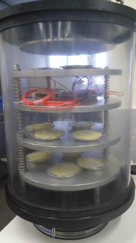
All the prepared samples were distributed in 1 cm thick aluminum plates and frozen. In the case of slow freezing curves, the samples were frozen for 48 hours at −45°C (Liebherr Medline, LCT 2325, Germany), and for the case of fast freezing curves, the samples were frozen at −45°C for 3 hours (Hiber RDM051S, Italy). Subsequently, both samples were stored in the Liebherr Medline freezer previously mentioned at −45°C until freeze-dried. The drying step was carried out using a Telstar Lyo Quest 55 (Terrassa, Spain) freeze-dryer operating at different shelf temperatures (30°C and 40°C) and 50 Pa. The samples in the drying chamber are shown in Figure 1.

Figure 1. Freeze drying chamber for orange juice based cake experimental dynamics.

Figura 1. Cámara de secado por congelación utilizada para las dinámicas experimentales de la torta con base de jugo naranja

Freeze-drying dynamics were carried out by weight loss every 3 h, until a stable humidity was reached. The measurement was made by triplicate in three different samples which were disposable for each point. Two sets of freeze-drying dynamics were obtained: set 1 performed without heat application to the heating plate and environmental temperature of 30°C; set 2 performed by heating the plate at 40°C with environmental temperature of 30 °C. Initial moisture of the sample prior to freeze-drying was evaluated by triplicate in a vacuum oven (Vaciotem-T 4001489, JP Selecta, Spain) at 60 ± 1°C and <100 mmHg, until reaching a constant weight in agreement with the official method 20.013 as was suggested by Uscanga et al. (2020). The effect of process variables on quality changes during orange juice-based cake freeze-drying are discussed in deep by Uscanga et al. (2020). In this study, the experimental freeze dynamics are used for Darcy’s pseudo permeability and deviation index evaluation.

3.2. Dimensionless analysis

In order to normalize the independent variables (time $t$ and coordinates $z_{\beta }$, $z_{\gamma }$) the following dimensionless variables and constants were introduced,

$\mathrm{\Phi }=\frac{X}{X_0}{\mathrm{\Psi }}_{\beta }=\frac{T_{\beta }-T_f}{T_0-T_f}{\mathrm{\Psi }}_{\gamma }=\frac{T_{\gamma }-T_f}{T_0-T_f}{\mathrm{\Psi }}_h=\frac{T_h-T_f}{T_0-T_f}{\mathrm{\Psi }}_{env}=\frac{T_{env}-T_f}{T_0-T_f}$

$\tau =\frac{{\alpha }_{\gamma }t}{l^2}{\xi }_{\gamma }=\frac{z_{\gamma }}{l}{\xi }_{\beta }=\frac{z_{\beta }}{l}B{i}_{\beta }=\frac{h_{\beta }l}{k_{\beta }}B{i}_{\gamma }=\frac{h_{\gamma }l}{k_{\gamma }}$

Dimensionless equations,

(1b) $\frac{d\mathrm{\Phi }}{d\tau }=-\frac{A{\rho }_{wv}{K}^{\ast }{l}^2}{X_0{\alpha }_{\gamma }{m}_{s0}{\mu }_{wv}{l}_{\gamma }^{1+n}}\left(p_{w_{\beta \gamma }}-p_{\mathrm{\infty }}\right)$(1b)

(5b) $\frac{\mathrm{\partial }{\mathrm{\Psi }}_{\beta }}{\mathrm{\partial }{\xi }_{\beta }}=B{i}_{\beta }\left({\mathrm{\Psi }}_{\beta }-{\mathrm{\Psi }}_h\right)\mathrm{a}\mathrm{t}{\xi }_{\beta }=0\mathrm{a}\mathrm{n}\mathrm{d}\tau >0$(5b)

(6b) $\frac{\mathrm{\partial }{\mathrm{\Psi }}_{\beta }}{\mathrm{\partial }\tau }=\frac{\mathrm{\partial }{\mathrm{\Psi }}_{\gamma }}{\mathrm{\partial }\tau }\mathrm{a}\mathrm{t}\xi =\frac{l_{\beta }}{l}\mathrm{a}\mathrm{n}\mathrm{d}\tau >0$(6b)

(7b) $-\left(\frac{k_{\beta }}{k_{\gamma }}\right)\frac{\mathrm{\partial }{\mathrm{\Psi }}_{\beta }}{\mathrm{\partial }{\xi }_{\beta }}+\frac{\mathrm{\partial }{\mathrm{\Psi }}_{\gamma }}{\mathrm{\partial }{\xi }_{\gamma }}=\frac{r_w{\lambda }_{f}l}{k_{\gamma }\left(T_0-T_f\right)}\mathrm{a}\mathrm{t}\xi =\frac{l_{\beta }}{l}\mathrm{a}\mathrm{n}\mathrm{d}\tau >0$(7b)

(8b) $\frac{\mathrm{\partial }{\mathrm{\Psi }}_{\beta }}{\mathrm{\partial }\tau }=\frac{{\alpha }_{\beta }}{{\alpha }_{\gamma }}\left(\frac{{\mathrm{\partial }}^2{\mathrm{\Psi }}_{\beta }}{\mathrm{\partial }{\xi }_{\beta }^2}\right)\mathrm{i}\mathrm{n}0\le {\xi }_{\beta }\le \frac{l}{l_{\beta }}\mathrm{a}\mathrm{n}\mathrm{d}\tau >0$(8b)

(9b) $\frac{\mathrm{\partial }{\mathrm{\Psi }}_{\gamma }}{\mathrm{\partial }\tau }=\left(\frac{{\mathrm{\partial }}^2{\mathrm{\Psi }}_{\gamma }}{\mathrm{\partial }{\xi }_{\gamma }^2}\right)\mathrm{i}\mathrm{n}\mathrm{a}\mathrm{n}\mathrm{d}\tau >0$(9b)

(10b) $-\frac{\mathrm{\partial }{\mathrm{\Psi }}_{\gamma }}{\mathrm{\partial }{\xi }_{\gamma }}=B{i}_{\gamma }\left({\mathrm{\Psi }}_{\gamma }-{\mathrm{\Psi }}_{env}\right)\mathrm{a}\mathrm{t}{\xi }_{\gamma }=1\mathrm{a}\mathrm{n}\mathrm{d}\tau >0$(10b)

(11b) $\frac{d\left(l_{\beta }/l\right)}{d\tau }=\frac{X_0{m}_{s0}}{lA{\rho }_{wi}}\frac{d\mathrm{\Phi }}{d\tau }$(11b)

3.3. Model solution

The heat transfer equations (Eqs. 5b(5b) $\frac{\mathrm{\partial }{\mathrm{\Psi }}_{\beta }}{\mathrm{\partial }{\xi }_{\beta }}=B{i}_{\beta }\left({\mathrm{\Psi }}_{\beta }-{\mathrm{\Psi }}_h\right)\mathrm{a}\mathrm{t}{\xi }_{\beta }=0\mathrm{a}\mathrm{n}\mathrm{d}\tau >0$(5b) -10b(10b) $-\frac{\mathrm{\partial }{\mathrm{\Psi }}_{\gamma }}{\mathrm{\partial }{\xi }_{\gamma }}=B{i}_{\gamma }\left({\mathrm{\Psi }}_{\gamma }-{\mathrm{\Psi }}_{env}\right)\mathrm{a}\mathrm{t}{\xi }_{\gamma }=1\mathrm{a}\mathrm{n}\mathrm{d}\tau >0$(10b) ) can be discretized in space coordinates to obtain the following system of $2\left(N+1\right)$ ordinary differential equations (ODE),

(5c) $\frac{{\mathrm{\Psi }}_{\beta 2}-{\mathrm{\Psi }}_{\beta 0}}{2\mathrm{\Delta }{\xi }_{\beta }}=B{i}_{\beta }\left({\mathrm{\Psi }}_{\beta 1}-{\mathrm{\Psi }}_h\right)\mathrm{a}\mathrm{t}j=1$(5c)

(6c) $\frac{d{\mathrm{\Psi }}_{\beta j}}{d\tau }=\frac{{\alpha }_{\beta }}{{\alpha }_{\gamma }}\left(\frac{{\mathrm{\Psi }}_{\beta j+1}-2{\mathrm{\Psi }}_{\beta j}+{\mathrm{\Psi }}_{\beta j-1}}{\mathrm{\Delta }{\xi }_{\beta }^2}\right)\mathrm{f}\mathrm{o}\mathrm{r}j=1,2,\cdot \cdot \cdot ,N+1$(6c)

(7c) $-\left(\frac{k_{\beta }}{k_{\gamma }}\right)\frac{{\mathrm{\Psi }}_{\beta N+2}-{\mathrm{\Psi }}_{\beta N}}{2\mathrm{\Delta }{\xi }_{\beta }}+\frac{{\mathrm{\Psi }}_{\gamma 2}-{\mathrm{\Psi }}_{\gamma 0}}{2\mathrm{\Delta }{\xi }_{\gamma }}=\frac{r_w{\lambda }_{f}l}{k_{\gamma }\left(T_0-T_f\right)}\mathrm{a}\mathrm{t}j=N+1\mathrm{a}\mathrm{n}\mathrm{d}i=1$(7c)

(8c) $\frac{{\alpha }_{\beta }}{{\alpha }_{\gamma }}\left(\frac{{\mathrm{\Psi }}_{\beta N+2}-2{\mathrm{\Psi }}_{\beta N+1}+{\mathrm{\Psi }}_{\beta N}}{\mathrm{\Delta }{\xi }_{\beta }^2}\right)=\frac{{\mathrm{\Psi }}_{\gamma 2}-2{\mathrm{\Psi }}_{\gamma 1}+{\mathrm{\Psi }}_{\gamma 0}}{\mathrm{\Delta }{\xi }_{\gamma }^2}\mathrm{a}\mathrm{t}j=N+1\mathrm{a}\mathrm{n}\mathrm{d}i=1$(8c)

(9c) $\frac{d{\mathrm{\Psi }}_{\gamma i}}{d\tau }=\frac{{\mathrm{\Psi }}_{\gamma i+1}-2{\mathrm{\Psi }}_{\gamma i}+{\mathrm{\Psi }}_{\gamma i-1}}{\mathrm{\Delta }{\xi }_{\gamma }^2}\mathrm{f}\mathrm{o}\mathrm{r}i=1,2,\cdot \cdot \cdot ,N+1$(9c)

(10c) $-\frac{{\mathrm{\Psi }}_{\gamma N+2}-{\mathrm{\Psi }}_{\gamma N}}{2\mathrm{\Delta }{\xi }_{\gamma }}=B{i}_{\gamma }\left({\mathrm{\Psi }}_{\gamma N+1}-{\mathrm{\Psi }}_{env}\right)\mathrm{a}\mathrm{t}i=N+1$(10c)

Where $\mathrm{\Delta }{\xi }_{\beta }=\frac{l_{\beta }/l}{N}$ and $\mathrm{\Delta }{\xi }_{\gamma }=\frac{l_{\gamma }/l}{N}$

Eqs. (5c)(5c) $\frac{{\mathrm{\Psi }}_{\beta 2}-{\mathrm{\Psi }}_{\beta 0}}{2\mathrm{\Delta }{\xi }_{\beta }}=B{i}_{\beta }\left({\mathrm{\Psi }}_{\beta 1}-{\mathrm{\Psi }}_h\right)\mathrm{a}\mathrm{t}j=1$(5c) -(10c(10c) $-\frac{{\mathrm{\Psi }}_{\gamma N+2}-{\mathrm{\Psi }}_{\gamma N}}{2\mathrm{\Delta }{\xi }_{\gamma }}=B{i}_{\gamma }\left({\mathrm{\Psi }}_{\gamma N+1}-{\mathrm{\Psi }}_{env}\right)\mathrm{a}\mathrm{t}i=N+1$(10c) ) can be numerically solved by any common method for ODEs. During freeze-drying sublimation front at $z=l_{\beta }$ is moving following Eq. (11b)(11b) $\frac{d\left(l_{\beta }/l\right)}{d\tau }=\frac{X_0{m}_{s0}}{lA{\rho }_{wi}}\frac{d\mathrm{\Phi }}{d\tau }$(11b) . However, in order to apply the analytical solution (Eq. 15(15) $X=\frac{l-{\left(\left(n+2\right)a_2{a}_1{K}^{\ast }t\right)}^{1/\left(n+2\right)}}{a_2}$(15) ), Eqs. (5c)(5c) $\frac{{\mathrm{\Psi }}_{\beta 2}-{\mathrm{\Psi }}_{\beta 0}}{2\mathrm{\Delta }{\xi }_{\beta }}=B{i}_{\beta }\left({\mathrm{\Psi }}_{\beta 1}-{\mathrm{\Psi }}_h\right)\mathrm{a}\mathrm{t}j=1$(5c) -(10c(10c) $-\frac{{\mathrm{\Psi }}_{\gamma N+2}-{\mathrm{\Psi }}_{\gamma N}}{2\mathrm{\Delta }{\xi }_{\gamma }}=B{i}_{\gamma }\left({\mathrm{\Psi }}_{\gamma N+1}-{\mathrm{\Psi }}_{env}\right)\mathrm{a}\mathrm{t}i=N+1$(10c) ) may be solved at constant $l_{\beta }=l/2$, in order to obtain a pseudo stationary average sublimation front temperature. Water loss rate ($r_w$) is required to solve the Eqs. (5c)(5c) $\frac{{\mathrm{\Psi }}_{\beta 2}-{\mathrm{\Psi }}_{\beta 0}}{2\mathrm{\Delta }{\xi }_{\beta }}=B{i}_{\beta }\left({\mathrm{\Psi }}_{\beta 1}-{\mathrm{\Psi }}_h\right)\mathrm{a}\mathrm{t}j=1$(5c) -(10c(10c) $-\frac{{\mathrm{\Psi }}_{\gamma N+2}-{\mathrm{\Psi }}_{\gamma N}}{2\mathrm{\Delta }{\xi }_{\gamma }}=B{i}_{\gamma }\left({\mathrm{\Psi }}_{\gamma N+1}-{\mathrm{\Psi }}_{env}\right)\mathrm{a}\mathrm{t}i=N+1$(10c) ) and therefore the estimation of $r_w$ in two cases will be discussed in section 3.4.

3.4. Analytical model application

Analytical solution (Eq. 15)(15) $X=\frac{l-{\left(\left(n+2\right)a_2{a}_1{K}^{\ast }t\right)}^{1/\left(n+2\right)}}{a_2}$(15) for freeze-drying dynamic may be applied in two cases: for pseudo Darcy’s permeability estimation from experimental results; or, for prediction of the freeze-drying time.

Case 1. In the case of pseudo Darcy’s permeability estimation by fitting to experimental results r_w may be estimated from.

(16) $r_w=-\frac{m_{s0}}{A}{\left(\frac{\mathrm{\Delta }X}{\mathrm{\Delta }t}\right)}_{exp}$(16)

Case 2. In the case of prediction freeze-drying time, an initial guess for sublimation front temperature ($T_{\beta \gamma }$) must be assumed (between ice water saturation temperature at work pressure $p_{wi}$ and 273.15 K). Eq. (15)(15) $X=\frac{l-{\left(\left(n+2\right)a_2{a}_1{K}^{\ast }t\right)}^{1/\left(n+2\right)}}{a_2}$(15) is solved with an initial guess and $r_w$ is estimated with Eq. (16(16) $r_w=-\frac{m_{s0}}{A}{\left(\frac{\mathrm{\Delta }X}{\mathrm{\Delta }t}\right)}_{exp}$(16) ) (the gradients are not experimental and they are obtained with Eq. 15)(15) $X=\frac{l-{\left(\left(n+2\right)a_2{a}_1{K}^{\ast }t\right)}^{1/\left(n+2\right)}}{a_2}$(15) . With an estimated $r_w$, Eqs. (5c)(5c) $\frac{{\mathrm{\Psi }}_{\beta 2}-{\mathrm{\Psi }}_{\beta 0}}{2\mathrm{\Delta }{\xi }_{\beta }}=B{i}_{\beta }\left({\mathrm{\Psi }}_{\beta 1}-{\mathrm{\Psi }}_h\right)\mathrm{a}\mathrm{t}j=1$(5c) -(10c(10c) $-\frac{{\mathrm{\Psi }}_{\gamma N+2}-{\mathrm{\Psi }}_{\gamma N}}{2\mathrm{\Delta }{\xi }_{\gamma }}=B{i}_{\gamma }\left({\mathrm{\Psi }}_{\gamma N+1}-{\mathrm{\Psi }}_{env}\right)\mathrm{a}\mathrm{t}i=N+1$(10c) ) are solved to calculate a sublimation front average pseudo stationary temperature. The procedure is repeated until convergence is obtained.

4. Results

4.1. Permeability and pseudo-permeability estimation

Heat transfer equations (Eqs. 5c(5c) $\frac{{\mathrm{\Psi }}_{\beta 2}-{\mathrm{\Psi }}_{\beta 0}}{2\mathrm{\Delta }{\xi }_{\beta }}=B{i}_{\beta }\left({\mathrm{\Psi }}_{\beta 1}-{\mathrm{\Psi }}_h\right)\mathrm{a}\mathrm{t}j=1$(5c) -10c(10c) $-\frac{{\mathrm{\Psi }}_{\gamma N+2}-{\mathrm{\Psi }}_{\gamma N}}{2\mathrm{\Delta }{\xi }_{\gamma }}=B{i}_{\gamma }\left({\mathrm{\Psi }}_{\gamma N+1}-{\mathrm{\Psi }}_{env}\right)\mathrm{a}\mathrm{t}i=N+1$(10c) ) were solved by ode15s Matlab routine at 30°C (set 1) in heating plate and $l_{\beta }=l/2$ with the complete variables and properties of set 1 experiment listed in Table 1. The experimental value of ${\left(\mathrm{\Delta }X/\mathrm{\Delta }t\right)}_{exp}$ for Eq (16)(16) $r_w=-\frac{m_{s0}}{A}{\left(\frac{\mathrm{\Delta }X}{\mathrm{\Delta }t}\right)}_{exp}$(16) was calculated with the 3 independent replicates accomplished for set 1 experiment. The temperature evolution obtained for frozen zone is plotted in Figure 2 and for dried (porous) zone in Figure 3. Figures 2 and Figure 3 show that as sublimation front and water loss are considered constant, the heat transfer equations reach a pseudo stationary temperature. This pseudo-stationary sublimation front temperature was −12.1°C. With this temperature, the average water vapor pressure and viscosity at sublimation front were calculated with Eqs. (3)(3) $p_{w{v}_{\beta \gamma }}=e^{-3168.8+83545/T_{\beta \gamma }+529.54ln\left(T_{\beta \gamma }\right)-1.359\times {10}^{-3}{T}_{\beta \gamma }^2}$(3) and (4(4) ${\mu }_{wv}=-8.20744\times {10}^{-6}+9.88333\times {10}^{-8}T$(4) ) and constants a₁ and a₂ were calculated with the detailed definitions for Eq. (14)(14) $\frac{dX}{dt}=-\frac{a_1{K}^{\ast }}{{\left(l-a_{2}X\right)}^{1+n}}\mathrm{o}\mathrm{r}-\frac{1}{a_2}{\int }_{X_0}^X{\left(l-a_{2}X\right)}^{1+n}d\left(-a_{2}X\right)=-a_1{K}_m{\int }_{0+}^{t}dt$(14) . Then, D’Arcy’s permeability (for ideal behavior $n=0$) and pseudo permeability (for non-ideal behavior $n>0$) were estimated by non-linear least squares. The results joint with all the variables are listed in Table 2 and the fitted equations joint with the three replicates of experimental set 1 are plotted in Figure 4. Darcy’s permeability ($K$) and pseudo-permeability ($K^{\ast }$) were statistically significant but non-ideal index $n$ was not. This means that, although non-ideal Darcy’s law fit better the experimental results, the differences between ideal and non-ideal behaviors are not greater enough than experimental dispersion. Anyway, Eq. (15)(15) $X=\frac{l-{\left(\left(n+2\right)a_2{a}_1{K}^{\ast }t\right)}^{1/\left(n+2\right)}}{a_2}$(15) represents the experimental freeze-drying dynamic adequately. The Eq. (1)(1) $\frac{dX}{dt}=-\frac{A{\rho }_{wv}K}{m_{s0}{\mu }_{wv}{l}_{\gamma }}\left(p_{w{v}_{\beta \gamma }}-p_{\mathrm{\infty }}\right)$(1) or (1a) or (14) singularity can be observed in Figure 4 (the derivative tends to $-\mathrm{\infty }$ when $t\to 0$), but do not have effect on Eq. (15)(15) $X=\frac{l-{\left(\left(n+2\right)a_2{a}_1{K}^{\ast }t\right)}^{1/\left(n+2\right)}}{a_2}$(15) because the integration was performed between 0+ to $t$. Therefore, Eq. (15)(15) $X=\frac{l-{\left(\left(n+2\right)a_2{a}_1{K}^{\ast }t\right)}^{1/\left(n+2\right)}}{a_2}$(15) represents a simplified equation to estimate Darcy’s permeability or pseudo permeability at averaged sublimation front temperature. It is important to remark that in Eq. (15(15) $X=\frac{l-{\left(\left(n+2\right)a_2{a}_1{K}^{\ast }t\right)}^{1/\left(n+2\right)}}{a_2}$(15) ) $X\to -\mathrm{\infty }$ when $t\to \mathrm{\infty }$. This is the result that freeze-drying water loss is function of pressure gradient between water vapor at sublimation front (greater than) and vacuum pressure. It is analog to water loss in a bowl with boiling water. If heat is continuously transferred to water in the bowl, the water keeps at boiling point while liquid water exists in bowl. When liquid water is exhausted, water loss no longer exists. In the same way, Eq. (15)(15) $X=\frac{l-{\left(\left(n+2\right)a_2{a}_1{K}^{\ast }t\right)}^{1/\left(n+2\right)}}{a_2}$(15) only exits while solid water keeps in the product, and therefore Eq. (15)(15) $X=\frac{l-{\left(\left(n+2\right)a_2{a}_1{K}^{\ast }t\right)}^{1/\left(n+2\right)}}{a_2}$(15) dominion is $X>0$. A reference for this dominion is indicated as a horizontal line in Figure 4. There is more water in vapor form in porous zone, but water vapor density is around 1/900 of solid water density and therefore for drying purposes may be considered zero. As can be observed in Figure 4, experimental results may produce negative moistures because the moisture was calculated by weight loss in different samples from which the initial moisture was determined. Negative experimental moistures indicate that final moisture is around zero.

Table 1. Variables and properties for heat transfer equations at experimental set 1.

Tabla 1. Variables y propiedades para las ecuaciones de transferencia de calor en el conjunto experimental 1

Variable/Property	Value	Reference
$N$	15	This study
$T_0$, $T_f$	−27, 30 ${\hspace{0.17em}}^{\mathrm{o}}\mathrm{C}$	Experimental
$T_h$, $T_{env}$	30, 30 ${\hspace{0.17em}}^{\mathrm{o}}\mathrm{C}$	Experimental
$A$, $l$	2.6x10^−3 ${\mathrm{m}}^2$, 0.01 $\mathrm{m}$	Experimental
$p_{\mathrm{\infty }}$	50 $\mathrm{P}\mathrm{a}$	Experimental
$m_{s0}$	5.4x10^−3 $\mathrm{k}\mathrm{g}$	Experimental
${\left(\mathrm{\Delta }X/\mathrm{\Delta }t\right)}_{exp}$	9.2x10^−5 $\mathrm{k}\mathrm{g}\mathrm{w}\cdot \mathrm{k}\mathrm{g}\mathrm{d}{\mathrm{m}}^{-1}\cdot {\mathrm{s}}^{-1}$	Experimental, averaged form three replicates.
$\mathrm{\Delta }{H}_s$	2.78X10^6 $\mathrm{J}\cdot \mathrm{k}{\mathrm{g}}^{-1}$	Geankoplis (1998)
$k_{\beta }$, $k_{\gamma }$	2.5, 0.15 $\mathrm{W}\cdot {\mathrm{m}}^{-1}\cdot \mathrm{k}{\mathrm{g}}^{-1}$	Lopez-Quiroga et al. (2012)
${\alpha }_{\beta }$, ${\alpha }_{\gamma }$	(5.2, 1.0)x10^−7 ${\mathrm{m}}^2\cdot {\mathrm{s}}^{-1}$	Lopez-Quiroga et al. (2012)
$h_{\beta }$, $h_{\gamma }$	8, 12 $\mathrm{W}\cdot {\mathrm{m}}^{-2}\cdot \mathrm{k}{\mathrm{g}}^{-1}$	Empirical correlations natural convection.

Table 2. Variables and fitted properties obtained by non-linear least squares of Eq. (15)(15) $X=\frac{l-{\left(\left(n+2\right)a_2{a}_1{K}^{\ast }t\right)}^{1/\left(n+2\right)}}{a_2}$(15) on experimental freeze drying kinetic at set 1.

Tabla 2. Variables y propiedades ajustadas obtenidas por mínimos cuadrados no lineales de la ec. (15) sobre la cinética de liofilización experimental del conjunto 1

Variable/Property	Value	Reference
$X_0$	4 $\mathrm{k}\mathrm{g}\mathrm{w}\mathrm{a}\mathrm{t}\mathrm{e}\mathrm{r}\cdot {\left(\mathrm{k}\mathrm{g}\mathrm{d}\mathrm{r}\mathrm{y}\mathrm{m}\mathrm{a}\mathrm{t}\mathrm{t}\mathrm{e}\mathrm{r}\right)}^{-1}$	Experimental, averaged of three independent replicates
$T_{i\beta \gamma }$	−12.1 ${\hspace{0.17em}}^{\mathrm{o}}\mathrm{C}$	Result for pseudo-stationary heat transfer
${\rho }_{wi}$	900 $\mathrm{k}\mathrm{g}\cdot {\mathrm{m}}^{-3}$	Geankoplis (1998)
$K$, $n=0$	2.50x10^−11 ${\mathrm{m}}^2$	Fitted
$K^{\ast }$, $n$	2.0x10^−12 ${\mathrm{m}}^{2.5}$, 0.5	Fitted

Figure 2. Temperature evolution in the 15 nodes of frozen zone obtained by solution of Eqs. (5c)(5c) $\frac{{\mathrm{\Psi }}_{\beta 2}-{\mathrm{\Psi }}_{\beta 0}}{2\mathrm{\Delta }{\xi }_{\beta }}=B{i}_{\beta }\left({\mathrm{\Psi }}_{\beta 1}-{\mathrm{\Psi }}_h\right)\mathrm{a}\mathrm{t}j=1$(5c) -(10c(10c) $-\frac{{\mathrm{\Psi }}_{\gamma N+2}-{\mathrm{\Psi }}_{\gamma N}}{2\mathrm{\Delta }{\xi }_{\gamma }}=B{i}_{\gamma }\left({\mathrm{\Psi }}_{\gamma N+1}-{\mathrm{\Psi }}_{env}\right)\mathrm{a}\mathrm{t}i=N+1$(10c) ) with $l_{\beta }=l/2$ at variables and properties listed in Table 1.

Figura 2. Evolución de la temperatura en los 15 nodos de la zona congelada obtenida por la solución de las ecuaciones (5 c)-(10 c) con$l_{\beta }=l/2$ en las variables y propiedades enumeradas en la Tabla 1

Figure 3. Temperature evolution in the 15 nodes of porous zone obtained by solution of Eqs. (5c)(5c) $\frac{{\mathrm{\Psi }}_{\beta 2}-{\mathrm{\Psi }}_{\beta 0}}{2\mathrm{\Delta }{\xi }_{\beta }}=B{i}_{\beta }\left({\mathrm{\Psi }}_{\beta 1}-{\mathrm{\Psi }}_h\right)\mathrm{a}\mathrm{t}j=1$(5c) -(10c(10c) $-\frac{{\mathrm{\Psi }}_{\gamma N+2}-{\mathrm{\Psi }}_{\gamma N}}{2\mathrm{\Delta }{\xi }_{\gamma }}=B{i}_{\gamma }\left({\mathrm{\Psi }}_{\gamma N+1}-{\mathrm{\Psi }}_{env}\right)\mathrm{a}\mathrm{t}i=N+1$(10c) ) with $l_{\beta }=l/2$ at variables and properties listed in Table 1.

Figura 3. Evolución de la temperatura en los 15 nodos de la zona porosa obtenida por la solución de las ecuaciones (5 c)-(10 c) con$l_{\beta }=l/2$ en las variables y propiedades enumeradas en la Tabla 1

Figure 4. Experimental (o) and fitted (lines) freeze drying dynamics at condition listed in Table 2. Discontinuous line represents the ideal Darcy’s Law (Eq. 15(15) $X=\frac{l-{\left(\left(n+2\right)a_2{a}_1{K}^{\ast }t\right)}^{1/\left(n+2\right)}}{a_2}$(15) with $n=0$) and continuous line the non-ideal one. (Horizontal line at zero moisture represents the physical limit for Eq. 15(15) $X=\frac{l-{\left(\left(n+2\right)a_2{a}_1{K}^{\ast }t\right)}^{1/\left(n+2\right)}}{a_2}$(15) domain).

Figura 4. Dinámica de liofilización experimental (o) y ajustada (líneas) en las condiciones enumeradas en la Tabla 2. La línea discontinua representa la ley de Darcy ideal (Ec. 15 con) y la línea continua la no-ideal. (La línea horizontal a humedad cero representa el límite físico para el dominio de la Ec. 15)

4.2. Freeze drying dynamic prediction

The Darcy’s permeability and pseudo permeability estimated and listed in Table 2 were used for the prediction of freeze-drying dynamic of the same orange juice bases cake but freeze-dried with 40°C in the heating plate (set 2 experiment). The complete heat transfer conditions of this second set of experiments are summarized in Table 3 and the complete moisture data are summarized in Table 4. As it was indicated for the case 2 of section 3.4, an initial guess for averaged sublimation front was required. Considering that in this second set of experiments the hot plate was operated at 40°C we assume a greater temperature than those obtained for the first set of experiment. The initial guess was −10.5°C (indicated in Table 3). With this temperature, the water vapor was calculated with Eq. (3)(3) $p_{w{v}_{\beta \gamma }}=e^{-3168.8+83545/T_{\beta \gamma }+529.54ln\left(T_{\beta \gamma }\right)-1.359\times {10}^{-3}{T}_{\beta \gamma }^2}$(3) and applied in Eq. (15)(15) $X=\frac{l-{\left(\left(n+2\right)a_2{a}_1{K}^{\ast }t\right)}^{1/\left(n+2\right)}}{a_2}$(15) to estimate ${\left(\mathrm{\Delta }X/\mathrm{\Delta }t\right)}_{exp}$ with the pseudo-permeability and the ideal deviation index listed in Table 2. The result for ${\left(\mathrm{\Delta }X/\mathrm{\Delta }t\right)}_{exp}$ is listed in Table 3. This initial guess and the variables listed in Table 3 were applied in heat transfer equations and the pseudo stationary state reached is plotted in Figures 5 and Figure 6. The averaged sublimation front pseudo stationary temperature was −9.7°C which is near than initial guess (−10.5°C). This temperature (−10.5°C) and the experimental values listed in Table 4 were applied in Eq. (15)(15) $X=\frac{l-{\left(\left(n+2\right)a_2{a}_1{K}^{\ast }t\right)}^{1/\left(n+2\right)}}{a_2}$(15) both for ideal and non-ideal Darcy’s law (with $K$, $K^{\ast }$ and $n$ listed in Table 2) to predict freeze-drying dynamic. Predicted and experimental results are plotted in Figure 7. Reference for Eq. (15)(15) $X=\frac{l-{\left(\left(n+2\right)a_2{a}_1{K}^{\ast }t\right)}^{1/\left(n+2\right)}}{a_2}$(15) dominion is represented in Figure 7 as horizontal line. Figure 7 shows that both ideal and non-ideal proposed analytical solution (Eq. 15)(15) $X=\frac{l-{\left(\left(n+2\right)a_2{a}_1{K}^{\ast }t\right)}^{1/\left(n+2\right)}}{a_2}$(15) for water loss during freeze-drying has prediction capacity at different conditions than those at which permeability and pseudo permeability were estimated. Non-ideal Darcy’s law produces better behavior predictions, but it wasn’t statistically significant with respect to ideal one.

Table 3. Variables and properties for heat transfer equations at experimental set 2.

Tabla 3. Variables y propiedades para las ecuaciones de transferencia de calor en el conjunto experimental 2

Variable/Property	Value	Reference
$N$	15	This study
$T_0$, $T_f$	−42, 40 ${\hspace{0.17em}}^{\mathrm{o}}\mathrm{C}$	Experimental
$T_h$, $T_{env}$	40, 30 ${\hspace{0.17em}}^{\mathrm{o}}\mathrm{C}$	Experimental
$A$, $l$	2.6x10^−3 ${\mathrm{m}}^2$, 0.01 $\mathrm{m}$	Experimental
$p_{\mathrm{\infty }}$	50 $\mathrm{P}\mathrm{a}$	Experimental
$m_{s0}$	4.6x10^−3 $\mathrm{k}\mathrm{g}$	Experimental
${\left(\mathrm{\Delta }X/\mathrm{\Delta }t\right)}_{exp}$	1.5x10^−4 $\mathrm{k}\mathrm{g}\mathrm{w}\cdot \mathrm{k}\mathrm{g}\mathrm{d}{\mathrm{m}}^{-1}\cdot {\mathrm{s}}^{-1}$	Initial guess at −10.5°C
$\mathrm{\Delta }{H}_s$	2.78X10^6 $\mathrm{J}\cdot \mathrm{k}{\mathrm{g}}^{-1}$	Geankoplis (1998)
$k_{\beta }$, $k_{\gamma }$	2.5, 0.15 $\mathrm{W}\cdot {\mathrm{m}}^{-1}\cdot \mathrm{k}{\mathrm{g}}^{-1}$	Lopez-Quiroga et al. (2012)
${\alpha }_{\beta }$, ${\alpha }_{\gamma }$	(5.2, 1.0)x10^−7 ${\mathrm{m}}^2\cdot {\mathrm{s}}^{-1}$	Lopez-Quiroga et al. (2012)
$h_{\beta }$, $h_{\gamma }$	14, 12 $\mathrm{W}\cdot {\mathrm{m}}^{-2}\cdot \mathrm{k}{\mathrm{g}}^{-1}$	Empirical correlations natural convection with conduction

Table 4. Variables and properties used for simulation of experimental freeze drying kinetic at set 2 with Eq. (15)(15) $X=\frac{l-{\left(\left(n+2\right)a_2{a}_1{K}^{\ast }t\right)}^{1/\left(n+2\right)}}{a_2}$(15) .

Tabla 4. Variables y propiedades utilizadas para la simulación de la cinética de liofilización experimental en el conjunto 2 con la ecuación (15)

Variable/Property	Value	Reference
$X_0$	4.9 $\mathrm{k}\mathrm{g}\mathrm{w}\mathrm{a}\mathrm{t}\mathrm{e}\mathrm{r}\cdot {\left(\mathrm{k}\mathrm{g}\mathrm{d}\mathrm{r}\mathrm{y}\mathrm{m}\mathrm{a}\mathrm{t}\mathrm{t}\mathrm{e}\mathrm{r}\right)}^{-1}$	Experimental, averaged of three independent replicates
$T_{i\beta \gamma }$	−9.7 ${\hspace{0.17em}}^{\mathrm{o}}\mathrm{C}$	Result for pseudo-stationary heat transfer
${\rho }_{wi}$	900 $\mathrm{k}\mathrm{g}\cdot {\mathrm{m}}^{-3}$	Geankoplis (1998)
$K$, $n=0$	2.50x10^−11 ${\mathrm{m}}^2$	Fitted
$K^{\ast }$, $n$	2.0x10^−12 ${\mathrm{m}}^{2.5}$, 0.5	Fitted

Figure 5. Temperature evolution in the 15 nodes of frozen zone obtained by solution of Eqs. (5c)(5c) $\frac{{\mathrm{\Psi }}_{\beta 2}-{\mathrm{\Psi }}_{\beta 0}}{2\mathrm{\Delta }{\xi }_{\beta }}=B{i}_{\beta }\left({\mathrm{\Psi }}_{\beta 1}-{\mathrm{\Psi }}_h\right)\mathrm{a}\mathrm{t}j=1$(5c) -(10c(10c) $-\frac{{\mathrm{\Psi }}_{\gamma N+2}-{\mathrm{\Psi }}_{\gamma N}}{2\mathrm{\Delta }{\xi }_{\gamma }}=B{i}_{\gamma }\left({\mathrm{\Psi }}_{\gamma N+1}-{\mathrm{\Psi }}_{env}\right)\mathrm{a}\mathrm{t}i=N+1$(10c) ) with $l_{\beta }=l/2$ at variables and properties listed in Table 3.

Figura 5. Evolución de la temperatura en los 15 nodos de la zona congelada obtenida por la solución de las ecuaciones (5 c)-(10 c) con$l_{\beta }=l/2$ en las variables y propiedades enumeradas en la Tabla 3

Figure 6. Temperature evolution in the 15 nodes of porous zone obtained by solution of Eqs (5c)(5c) $\frac{{\mathrm{\Psi }}_{\beta 2}-{\mathrm{\Psi }}_{\beta 0}}{2\mathrm{\Delta }{\xi }_{\beta }}=B{i}_{\beta }\left({\mathrm{\Psi }}_{\beta 1}-{\mathrm{\Psi }}_h\right)\mathrm{a}\mathrm{t}j=1$(5c) -(10c(10c) $-\frac{{\mathrm{\Psi }}_{\gamma N+2}-{\mathrm{\Psi }}_{\gamma N}}{2\mathrm{\Delta }{\xi }_{\gamma }}=B{i}_{\gamma }\left({\mathrm{\Psi }}_{\gamma N+1}-{\mathrm{\Psi }}_{env}\right)\mathrm{a}\mathrm{t}i=N+1$(10c) ) with $l_{\beta }=l/2$ at variables and properties listed in Table 3.

Figura 6. Evolución de la temperatura en los 15 nodos de la zona porosa obtenida por la solución de las ecuaciones (5 c)-(10 c) con$l_{\beta }=l/2$ en las variables y propiedades enumeradas en la Tabla 3

Figure 7. Experimental (o) and predicted (lines) freeze drying dynamics at condition listed in Table 4. Discontinuous line represents the ideal Darcy’s law (Eq. 15(15) $X=\frac{l-{\left(\left(n+2\right)a_2{a}_1{K}^{\ast }t\right)}^{1/\left(n+2\right)}}{a_2}$(15) with $n=0$) and continuous line the non-ideal one. (Horizontal line at zero moisture represents the physical limit for Eq. 15(15) $X=\frac{l-{\left(\left(n+2\right)a_2{a}_1{K}^{\ast }t\right)}^{1/\left(n+2\right)}}{a_2}$(15) domain).

Figura 7. Dinámicas de liofilización experimental (o) y predicha (líneas) en las condiciones enumeradas en la Tabla 4. La línea discontinua representa la ley de Darcy ideal (Ec. 15 con n = 0) y la línea continua la no-ideal. (La línea horizontal a humedad cero representa el límite físico para el dominio de la Ec. 15)

Therefore, proposed equation is an analytical equation that can be used to estimate averaged Darcy’s permeability in foods during freeze-drying. Taking into account that numerical solution of Eq. (1)(1) $\frac{dX}{dt}=-\frac{A{\rho }_{wv}K}{m_{s0}{\mu }_{wv}{l}_{\gamma }}\left(p_{w{v}_{\beta \gamma }}-p_{\mathrm{\infty }}\right)$(1) fails (numerical solution must be started at an arbitrary t > 0 with an arbitrary l_γ>0) at initial stages, the proposed model represents an alternative for modeling. The prediction capacity of proposed model depends on the sublimation front averaged temperature and the Darcy’s law properties ($K$ or $K^{\ast }$ and $n$). The sublimation front averaged temperature may be estimated as it was detailed in section 3.4. case 2. But $K$ or $K^{\ast }$ and $n$ requires non-linear regression estimation on experimental freeze-drying dynamic of a given product.

5. Conclusions

An analytical solution for Darcy’s law-based mathematical modeling of water loss dynamic during freeze-drying was proposed. Obtained equation resolves the mass transfer singularity produced by zero thickness of dried zone at time zero. The proposed analytical solution requires the complement of numerical solution of heat transfer equations with an averaged sublimation front position in sample. The proposed model was applied in the freeze-drying dynamic modeling of an orange juice-based cake. Darcy’s permeability was estimated both for ideal and non-ideal behavior and their prediction capacity for freeze-drying dynamic was shown. More work must be done to solve the singularity for heat transfer equations.

Nomenclature

$A$	=	Product cross section ${\mathrm{m}}^2$
$D$	=	Product diameter $\mathrm{m}$
$h$	=	Heat transfer coefficient $\mathrm{W}\cdot {\mathrm{m}}^{-1}\cdot {\mathrm{s}}^{-1}$
$k$	=	Heat conductivity $\mathrm{W}\cdot {\mathrm{m}}^{-1}\cdot {\mathrm{s}}^{-1}$
$K$	=	Dried product Darcy’s permeability ${\mathrm{m}}^2$
$K^{\ast }$	=	Dried product Darcy’s pseudo permeability ${\mathrm{m}}^{2+n}$
$l$	=	Product thickness $\mathrm{m}$
$m$	=	Mass $\mathrm{k}\mathrm{g}$
$n$	=	ideal deviation index
$p$	=	Pressure $\mathrm{P}\mathrm{a}$
$r$	=	Mass loss rate $\mathrm{k}\mathrm{g}\cdot {\mathrm{s}}^{-1}$
$t$	=	Time $\mathrm{s}$
$T$	=	Temperature $\mathrm{K}\mathrm{o}\mathrm{r}{\hspace{0.17em}}^{\mathrm{o}}\mathrm{C}$
$X$	=	Dry basis moisture $\mathrm{k}\mathrm{g}\mathrm{w}\mathrm{a}\mathrm{t}\mathrm{e}\mathrm{r}\cdot {\left(\mathrm{k}\mathrm{g}\mathrm{d}\mathrm{r}\mathrm{y}\mathrm{m}\mathrm{a}\mathrm{t}\mathrm{t}\mathrm{e}\mathrm{r}\right)}^{-1}$
$z$	=	Rectangular coordinate $\mathrm{m}$

Greek symbols	=
$\alpha$	=	Thermal diffusivity ${\mathrm{m}}^2\cdot {\mathrm{s}}^{-1}$
$\lambda$	=	Sublimation latent heat $\mathrm{J}\cdot \mathrm{k}{\mathrm{g}}^{-1}$
$\mu$	=	Viscosity $\mathrm{P}\mathrm{a}\cdot \mathrm{s}$
$\rho$	=	Density $\mathrm{k}\mathrm{g}\cdot {\mathrm{m}}^{-3}$

Subscripts	=
$0$	=	At initial ($t=0$)
$\mathrm{\infty }$	=	In vacuum tramp
$env$	=	For environmental
$f$	=	At final
$h$	=	For hot plate
$s$	=	For dry matter
$w$	=	For water
$wi$	=	For water ice
$wv$	=	For water vapor
$\beta$	=	In freeze product zone
$\gamma$	=	In porous (dried) product zone

Dimensionless groups	=
$Bi$	=	Biot number
$\mathrm{\Phi }$	=	Dimensionless moisture
$\tau$	=	Fourier number
$\xi$	=	Dimensionless coordinate
$\mathrm{\Psi }$	=	Dimensionless temperature

Disclosure

Authors confirm that there are no known conflicts of interest associated with this publication and the entire financial support for this work has been recognized in acknowledgements.

Acknowledgements

Authors express their acknowledgment to Mexican Consejo Nacional de Ciencia y Tecnología (CONACyT) for the scholarship of Uscanga-Ramos, M.A. (CVU No 469952); and Spanish Ministerio de Economía, Industria y Competitividad (Project AGL 2017-89251-R (AEI/FEDER-UE)) by its financial support.

Additional information

Funding

This work was supported by the Consejo Nacional de Ciencia y Tecnología (CONACyT) [CVU No 469952]; Ministerio de Economía, Industria y Competitividad [AGL 2017-89251-R].

References

- Bruttini, R., Rovero, G., & Baldi, G. (1991). Experimentation and modelling of pharmaceutical lyophilization using a pilot plant. The Chemical Engineering Journal, 45(3), 175–177. https://doi.org/https://doi.org/10.1016/0300-9467(91)80022-O
- Deepak, B., & Iqbal, Z. (2015). Lyophilization - Process and optimization for pharmaceuticals. International Journal of Drug Regulatory Affairs, 3(1), 30–40. https://doi.org/https://doi.org/10.22270/ijdra.v3i1.156
- Geankoplis, C. J. (1998). Procesos de transporte y operaciones unitarias (3th ed.). México, D.F: CECSA
- George, J. P., & Datta, A. K. (2002). Development and validation of heat and mass transfer models for freeze-drying of vegetable slices. Journal of Food Engineering, 52(1), 89–93. https://doi.org/https://doi.org/10.1016/S0260-8774(01)00091-7
- Henríquez, M., Almonacid, S., Lutz, M., Simpson, R., & Valdenegrob, M. (2013). Comparison of three drying processes to obtain an apple peel food ingredient. CYTA-Journal of Food, 11(2), 127–135. https://doi.org/https://doi.org/10.1080/19476337.2012.703693
- Leyva-Mayorga, M. A., Ramírez, J. A., Martín-Polo, M. O., Hernández, H. G., & Vázquez, M. (2002). Use of freeze-dried surimi in low-fat meat emulsions. CYTA-Journal of Food, 3(5), 288–294. https://doi.org/https://doi.org/10.1080/11358120209487741
- Liapis, A. I., & Bruttini, R. (1994). A theory for the primary and secondary drying stages of the freeze-drying of pharmaceutical crystalline and amorphous solutes: Comparison between experimental data and theory. Separation Technology, 4(3), 144–155. https://doi.org/https://doi.org/10.1016/0956-9618(94)80017-0
- Liapis, A. I., & Litchfield, R. J. (1979). Optimal control of a freeze dryer–I Theoretical development and quasi steady state analysis. Chemical Engineering Science, 34(7), 975–981. https://doi.org/https://doi.org/10.1016/0009-2509(79)85009-5
- Lopez-Quiroga, E., Antelo, L. T., & Alonso, A. A. (2012). Time-scale modeling and optimal control of freeze–drying. Journal of Food Engineering, 111(4), 655–666. https://doi.org/https://doi.org/10.1016/j.jfoodeng.2012.03.001
- Mascarenhasa, W. J., Akayavby, H. U., & Pikal, M. J. (1997). A computational model for finite element analysis of the freeze-drying process. Computer Methods in Applied Mechanics Engineering, 148(1–2), 105–124. https://doi.org/https://doi.org/10.1016/S0045-7825(96)00078-3
- Silva-Espinoza, M. A., Ayed, C., Foster, T., Camacho, M. D. M., & Martinez-Navarrete, N. (2020). The impact of freeze-Drying conditions on the physico-chemical properties and bioactive compounds of a freeze-dried orange puree. Foods, 9(1), 32,1–15. https://doi.org/https://doi.org/10.3390/foods9010032
- Uscanga, M. A., Camacho, M. M., Salgado, M. A., & Martinez-Navarrete, N. (2020). Influence of an orange product composition on the characteristics of the obtained freeze-dried cake and powder as related to their consumption pattern. Food and Bioprocess Technology, 13(8), 1368–1379. https://doi.org/https://doi.org/10.1007/s11947-020-02485-y